9   Routing-Update Algorithms

How do IP routers build and maintain their forwarding tables?

Ethernet bridges can always fall back on broadcast, so they can afford to build their forwarding tables “incrementally”, putting a host into the forwarding table only when that host is first seen as a sender. For IP, there is no fallback delivery mechanism: forwarding tables must be built before delivery can succeed. While manual table construction is possible, it is not practical.

In the literature it is common to refer to router-table construction as “routing algorithms”. We will avoid that term, however, to avoid confusion with the fundamental datagram-forwarding algorithm; instead, we will call these “routing-update algorithms”.

The two classes of algorithms we will consider here are distance-vector and link-state. Both assume that consistent information is available as to the cost of each link (eg that the two routers at opposite ends of each link know this cost). This requirement classifies these algorithms as interior routing-update algorithms: the routers involved are internal to a larger organization or other common administrative regime that has an established policy on how to assign link weights. The set of routers following a common policy is known as a routing domain or (from the BGP protocol) an autonomous system. The simplest link-weight strategy is to give each link a cost of 1; link costs can also be based on bandwidth, propagation delay, financial cost, or administrative preference value.

In the following chapter we will look at the Border Gateway Protocol, or BGP, in which no link-cost calculations are made, because links may be between unrelated organizations which have no agreement in place on determining link cost.

Generally, all these algorithms apply to IPv6 as well as IPv4, though specific protocols of course may need modification.

Finally, we should point out that from the early days of the Internet, routing was allowed to depend not just on the destination, but also on the “quality of service” (QoS) requested; thus, forwarding table entries are strictly speaking not ⟨destination, next_hop⟩ but rather ⟨destination, QoS, next_hop⟩. Originally, the Type of Service field in the IPv4 header (7.1   The IPv4 Header) could be used to specify QoS. Packets could request low delay, high throughput or high reliability, and could be routed accordingly. In practice, the Type of Service field was rarely used, and was eventually taken over by the DS field and ECN bits. The first three bits of the Type of Service field, known as the precedence bits, remain available, however, and can still be used for QoS routing purposes (see the Class Selector PHB of 18.7   Differentiated Services for examples of these bits). See also RFC 2386.

In much of the following, we are going to ignore QoS information, and assume that routing decisions are based only on the destination. See, however, the first paragraph of 9.5   Link-State Routing-Update Algorithm, and also 9.6   Routing on Other Attributes.

9.1   Distance-Vector Routing-Update Algorithm

Distance-Vector is the simplest routing-update algorithm, used by the Routing Information Protocol, or RIP. On unix-based systems the process in charge of this is often called “routed” (pronounced route-d).

Routers identify their router neighbors (through some sort of neighbor-discovery mechanism), and add a third column to their forwarding tables for cost; table entries are thus of the form ⟨destination,next_hop,cost⟩. The simplest case is to assign a cost of 1 to each link (the “hopcount” metric); it is also possible to assign more complex numbers.

Each router then reports the ⟨destination,cost⟩ portion of its table to its neighboring routers at regular intervals (these table portions are the “vectors” of the algorithm name). It does not matter if neighbors exchange reports at the same time, or even at the same rate.

Each router also monitors its continued connectivity to each neighbor; if neighbor N becomes unreachable then its reachability cost is set to infinity.

Actual destinations in IP would be networks attached to routers; one router might be directly connected to several such destinations. In the following, however, we will identify all a router’s directly connected networks with the router itself. That is, we will build forwarding tables to reach every router. While it is possible that one destination network might be reachable by two or more routers, thus breaking our identification of a router with its set of attached networks, in practice this is of little concern.

9.1.1   Distance-Vector Update Rules

Let A be a router receiving a report ⟨D,c_D⟩ from neighbor N at distance c_N. Note that this means A can reach D via N with cost c = c_D + c_N. A updates its own table according to the following three rules:

1. New destination: D is a previously unknown destination. A adds ⟨D,N,c_D+c_N⟩
2. Lower cost: D is a known destination with entry ⟨D,M,c⟩, but c > c_D+c_N. A updates the entry for D to ⟨D,N,c_D+c_N⟩. It is possible that M=N, meaning that N is now reporting a distance decrease to D.
3. Next_hop increase: A has a previous entry ⟨D,N,c⟩, but c < c_D+c_N. A updates the entry for D to ⟨D,N,c_D+c_N⟩. N is A’s next_hop to D, and N is now reporting a distance increase.

The first two rules are for new destinations and a shorter path to existing destinations. In these cases, the cost to each destination monotonically decreases (at least if we consider all unreachable destinations as being at distance ∞). Convergence is automatic, as the costs cannot decrease forever.

The third rule, however, introduces the possibility of instability, as a cost may also go up. It represents the bad-news case, in that neighbor N has learned that some link failure has driven up its own cost to reach D, and is now passing that “bad news” on to A, which routes to D via N.

The next_hop-increase case only passes bad news along; the very first cost increase must always come from a router discovering that a neighbor N is unreachable, and thus updating its cost to N to ∞. Similarly, if router A learns of a next_hop increase to destination D from neighbor B, then we can follow the next_hops back until we reach a router C which is either the originator of the cost=∞ report, or which has learned of an alternative route through one of the first two rules.

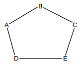
9.1.2   Example 1

For our first example, no links will break and thus only the first two rules above will be used. We will start out with the network below with empty forwarding tables; all link costs are 1.

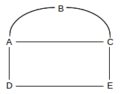
After initial neighbor discovery, here are the forwarding tables. Each node has entries only for its directly connected neighbors:

A: ⟨B,B,1⟩ ⟨C,C,1⟩ ⟨D,D,1⟩

B: ⟨A,A,1⟩ ⟨C,C,1⟩

C: ⟨A,A,1⟩ ⟨B,B,1⟩ ⟨E,E,1⟩

D: ⟨A,A,1⟩ ⟨E,E,1⟩

E: ⟨C,C,1⟩ ⟨D,D,1⟩

Now let D report to A; it sends records ⟨A,1⟩ and ⟨E,1⟩. A ignores D’s ⟨A,1⟩ record, but ⟨E,1⟩ represents a new destination; A therefore adds ⟨E,D,2⟩ to its table. Similarly, let A now report to D, sending ⟨B,1⟩ ⟨C,1⟩ ⟨D,1⟩ ⟨E,2⟩ (the last is the record we just added). D ignores A’s records ⟨D,1⟩ and ⟨E,2⟩ but A’s records ⟨B,1⟩ and ⟨C,1⟩ cause D to create entries ⟨B,A,2⟩ and ⟨C,A,2⟩. A and D’s tables are now, in fact, complete.

Now suppose C reports to B; this gives B an entry ⟨E,C,2⟩. If C also reports to E, then E’s table will have ⟨A,C,2⟩ and ⟨B,C,2⟩. The tables are now:

A: ⟨B,B,1⟩ ⟨C,C,1⟩ ⟨D,D,1⟩ ⟨E,D,2⟩

B: ⟨A,A,1⟩ ⟨C,C,1⟩ ⟨E,C,2⟩

C: ⟨A,A,1⟩ ⟨B,B,1⟩ ⟨E,E,1⟩

D: ⟨A,A,1⟩ ⟨E,E,1⟩ ⟨B,A,2⟩ ⟨C,A,2⟩

E: ⟨C,C,1⟩ ⟨D,D,1⟩ ⟨A,C,2⟩ ⟨B,C,2⟩

We have two missing entries: B and C do not know how to reach D. If A reports to B and C, the tables will be complete; B and C will each reach D via A at cost 2. However, the following sequence of reports might also have occurred:

• E reports to C, causing C to add ⟨D,E,2⟩
• C reports to B, causing B to add ⟨D,C,3⟩

In this case we have 100% reachability but B routes to D via the longer-than-necessary path B–C–E–D. However, one more report will fix this: suppose A reports to B. B will received ⟨D,1⟩ from A, and will update its entry ⟨D,C,3⟩ to ⟨D,A,2⟩.

Note that A routes to E via D while E routes to A via C; this asymmetry was due to indeterminateness in the selection of initial table exchanges.

If all link weights are 1, and if each pair of neighbors exchange tables once before any pair starts a second exchange, then the above process will discover the routes in order of length, ie the shortest paths will be the first to be discovered. This is not, however, a particularly important consideration.

9.1.3   Example 2

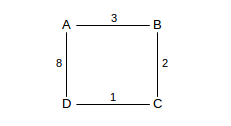
The next example illustrates link weights other than 1. The first route discovered between A and B is the direct route with cost 8; eventually we discover the longer A–C–D–B route with cost 2+1+3=6.

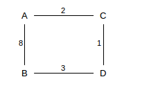
The initial tables are these:

A: ⟨C,C,2⟩ ⟨B,B,8⟩

B: ⟨A,A,8⟩ ⟨D,D,3⟩

C: ⟨A,A,2⟩ ⟨D,D,1⟩

D: ⟨B,B,3⟩ ⟨C,C,1⟩

After A and C exchange, A has ⟨D,C,3⟩ and C has ⟨B,A,10⟩. After C and D exchange, C updates its ⟨B,A,10⟩ entry to ⟨B,D,4⟩ and D adds ⟨A,C,3⟩; D receives C’s report of ⟨B,10⟩ but ignores it. Now finally suppose B and D exchange. D ignores B’s route to A, as it has a better one. B, however, gets D’s report ⟨A,3⟩ and updates its entry for A to ⟨A,D,6⟩. At this point the tables are as follows:

A: ⟨C,C,2⟩ ⟨B,B,8⟩ ⟨D,C,3⟩

B: ⟨A,D,6⟩ ⟨D,D,3⟩

C: ⟨A,A,2⟩ ⟨D,D,1⟩ ⟨B,D,4⟩

D: ⟨B,B,3⟩ ⟨C,C,1⟩ ⟨A,C,3⟩

We have two more things to fix before we are done: A has an inefficient route to B, and B has no route to C. The first will be fixed when C reports ⟨B,4⟩ to A; A will replace its route to B with ⟨B,C,6⟩. The second will be fixed when D reports to B; if A reports to B first then B will temporarily add the inefficient route ⟨C,A,10⟩; this will change to ⟨C,D,4⟩ when D’s report to B arrives. If we look only at the A–B route, B discovers the lower-cost route to A once, first, C reports to D and, second, after that, D reports to B; a similar sequence leads to A’s discovering the lower-cost route.

9.1.4   Example 3

Our third example will illustrate how the algorithm proceeds when a link breaks. We return to the first diagram, with all tables completed, and then suppose the D–E link breaks. This is the “bad-news” case: a link has broken, and is no longer available; this will bring the third rule into play.

We shall assume, as above, that A reaches E via D, but we will here assume – contrary to Example 1 – that C reaches D via A.

Initially, upon discovering the break, D and E update their tables to ⟨E,-,∞⟩ and ⟨D,-,∞⟩ respectively (whether or not they actually enter ∞ into their tables is implementation-dependent; we may consider this as equivalent to removing their entries for one another; the “-” as next_hop indicates there is no next_hop).

Eventually D and E will report the break to their respective neighbors A and C. A will apply the “bad-news” rule above and update its entry for E to ⟨E,-,∞⟩. We have assumed that C, however, routes to D via A, and so it will ignore E’s report.

We will suppose that the next steps are for C to report to E and to A. When C reports its route ⟨D,2⟩ to E, E will add the entry ⟨D,C,3⟩, and will again be able to reach D. When C reports to A, A will add the route ⟨E,C,2⟩. The final step will be when A next reports to D, and D will have ⟨E,A,3⟩. Connectivity is restored.

9.1.5   Example 4

The previous examples have had a “global” perspective in that we looked at the entire network. In the next example, we look at how one specific router, R, responds when it receives a distance-vector report from its neighbor S. Neither R nor S nor we have any idea of what the entire network looks like. Suppose R’s table is initially as follows, and the S–R link has cost 1:

destination	cost	next_hop
A	3	S
B	4	T
C	5	S
D	6	U

S now sends R the following report, containing only destinations and its costs:

destination	cost
A	2
B	3
C	5
D	4
E	2

R then updates its table as follows:

destination	cost	next_hop	reason
A	3	S	No change; S probably sent this report before
B	4	T	No change; R’s cost via S is tied with R’s cost via T
C	6	S	Next_hop increase
D	5	S	Lower-cost route via S
E	3	S	New destination

Whatever S’s cost to a destination, R’s cost to that destination via S is one greater.

9.2   Distance-Vector Slow-Convergence Problem

There is a significant problem with Distance-Vector table updates in the presence of broken links. Not only can routing loops form, but the loops can persist indefinitely! As an example, suppose we have the following arrangement, with all links having cost 1:

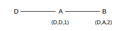
Now suppose the D–A link breaks:

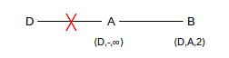
If A immediately reports to B that D is no longer reachable (distance = ∞), then all is well. However, it is possible that B reports to A first, telling A that it has a route to D, with cost 2, which B still believes it has.

This means A now installs the entry ⟨D,B,3⟩. At this point we have what we called in 1.6   Routing Loops a linear routing loop: if a packet is addressed to D, A will forward it to B and B will forward it back to A.

Worse, this loop will be with us a while. At some point A will report ⟨D,3⟩ to B, at which point B will update its entry to ⟨D,A,4⟩. Then B will report ⟨D,4⟩ to A, and A’s entry will be ⟨D,B,5⟩, etc. This process is known as slow convergence to infinity. If A and B each report to the other once a minute, it will take 2,000 years for the costs to overflow an ordinary 32-bit integer.

9.2.1   Slow-Convergence Fixes

The simplest fix to this problem is to use a small value for infinity. Most flavors of the RIP protocol use infinity=16, with updates every 30 seconds. The drawback to so small an infinity is that no path through the network can be longer than this; this makes paths with weighted link costs difficult. Cisco IGRP uses a variable value for infinity up to a maximum of 256; the default infinity is 100.

There are several well-known other fixes:

9.2.1.1   Split Horizon

Under split horizon, if A uses N as its next_hop for destination D, then A simply does not report to N that it can reach D; that is, in preparing its report to N it first deletes all entries that have N as next_hop. In the example above, split horizon would mean B would never report to A about the reachability of D because A is B’s next_hop to D.

Split horizon prevents all linear routing loops. However, there are other topologies where it cannot prevent loops. One is the following:

Suppose the A-D link breaks, and A updates to ⟨D,-,∞⟩. A then reports ⟨D,∞⟩ to B, which updates its table to ⟨D,-,∞⟩. But then, before A can also report ⟨D,∞⟩ to C, C reports ⟨D,2⟩ to B. B then updates to ⟨D,C,3⟩, and reports ⟨D,3⟩ back to A; neither this nor the previous report violates split-horizon. Now A’s entry is ⟨D,B,4⟩. Eventually A will report to C, at which point C’s entry becomes ⟨D,A,5⟩, and the numbers keep increasing as the reports circulate counterclockwise. The actual routing proceeds in the other direction, clockwise.

Split horizon often also includes poison reverse: if A uses N as its next_hop to D, then A in fact reports ⟨D,∞⟩ to N, which is a more definitive statement that A cannot reach D by itself. However, coming up with a scenario where poison reverse actually affects the outcome is not trivial.

9.2.1.2   Triggered Updates

In the original example, if A was first to report to B then the loop resolved immediately; the loop occurred if B was first to report to A. Nominally each outcome has probability 50%. Triggered updates means that any router should report immediately to its neighbors whenever it detects any change for the worse. If A reports first to B in the first example, the problem goes away. Similarly, in the second example, if A reports to both B and C before B or C report to one another, the problem goes away. There remains, however, a small window where B could send its report to A just as A has discovered the problem, before A can report to B.

9.2.1.3   Hold Down

Hold down is sort of a receiver-side version of triggered updates: the receiver does not use new alternative routes for a period of time (perhaps two router-update cycles) following discovery of unreachability. This gives time for bad news to arrive. In the first example, it would mean that when A received B’s report ⟨D,2⟩, it would set this aside. It would then report ⟨D,∞⟩ to B as usual, at which point B would now report ⟨D,∞⟩ back to A, at which point B’s earlier report ⟨D,2⟩ would be discarded. A significant drawback of hold down is that legitimate new routes are also delayed by the hold-down period.

These mechanisms for preventing slow convergence are, in the real world, quite effective. The Routing Information Protocol (RIP, RFC 2453) implements all but hold-down, and has been widely adopted at smaller installations.

However, the potential for routing loops and the limited value for infinity led to the development of alternatives. One alternative is the link-state strategy, 9.5   Link-State Routing-Update Algorithm. Another alternative is Cisco’s Enhanced Interior Gateway Routing Protocol, or EIGRP, 9.4.2   EIGRP. While part of the distance-vector family, EIGRP is provably loop-free, though to achieve this it must sometimes suspend forwarding to some destinations while tables are in flux.

9.3   Observations on Minimizing Route Cost

Does distance-vector routing actually achieve minimum costs? For that matter, does each packet incur the cost its sender expects? Suppose node A has a forwarding entry ⟨D,B,c⟩, meaning that A forwards packets to destination D via next_hop B, and expects the total cost to be c. If A sends a packet to D, and we follow it on the actual path it takes, must the total link cost be c? If so, we will say that the network has accurate costs.

The answer to the accurate-costs question, as it turns out, is yes for the distance-vector algorithm, if we follow the rules carefully, and the network is stable (meaning that no routing reports are changing, or, more concretely, that every update report now circulating is based on the current network state); a proof is below. However, if there is a routing loop, the answer is of course no: the actual cost is now infinite. The answer would also be no if A’s neighbor B has just switched to using a longer route to D than it last reported to A.

It turns out, however, that we seek the shortest route not because we are particularly trying to save money on transit costs; a route 50% longer would generally work just fine. (AT&T, back when they were the Phone Company, once ran a series of print advertisements claiming longer routes as a feature: if the direct path was congested, they could still complete your call by routing you the long way ‘round.) However, we are guaranteed that if all routers seek the shortest route – and if the network is stable – then all paths are loop-free, because in this case the network will have accurate costs.

Here is a simple example illustrating the importance of global cost-minimization in preventing loops. Suppose we have a network like this one:

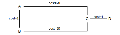
Now suppose that A and B use distance-vector but are allowed to choose the shortest route to within 10%. A would get a report from C that D could be reached with cost 1, for a total cost of 21. The forwarding entry via C would be ⟨D,C,21⟩. Similarly, A would get a report from B that D could be reached with cost 21, for a total cost of 22: ⟨D,B,22⟩. Similarly, B has choices ⟨D,C,21⟩ and ⟨D,A,22⟩.

If A and B both choose the minimal route, no loop forms. But if A and B both use the 10%-overage rule, they would be allowed to choose the other route: A could choose ⟨D,B,22⟩ and B could choose ⟨D,A,22⟩. If this happened, we would have a routing loop: A would forward packets for D to B, and B would forward them right back to A.

As we apply distance-vector routing, each router independently builds its tables. A router might have some notion of the path its packets would take to their destination; for example, in the case above A might believe that with forwarding entry ⟨D,B,22⟩ its packets would take the path A–B–C–D (though in distance-vector routing, routers do not particularly worry about the big picture). Consider again the accurate-cost question above. This fails in the 10%-overage example, because the actual path is now infinite.

We now prove that, in distance-vector routing, the network will have accurate costs, provided

• each router selects what it believes to be the shortest path to the final destination, and
• the network is stable, meaning that further dissemination of any reports would not result in changes

To see this, suppose the actual route taken by some packet from source to destination, as determined by application of the distributed algorithm, is longer than the cost calculated by the source. Choose an example of such a path with the fewest number of links, among all such paths in the network. Let S be the source, D the destination, and k the number of links in the actual path P. Let S’s forwarding entry for D be ⟨D,N,c⟩, where N is S’s next_hop neighbor. To have obtained this route through the distance-vector algorithm, S must have received report ⟨D,c_D⟩ from N, where we also have the cost of the S–N link as c_N and c = c_D + c_N. If we follow a packet from N to D, it must take the same path P with the first link deleted; this sub-path has length k-1 and so, by our hypothesis that k was the length of the shortest path with non-accurate costs, the cost from N to D is c_D. But this means that the cost along path P, from S to D via N, must be c_D + c_N = c, contradicting our selection of P as a path longer than its advertised cost.

There is one final observation to make about route costs: any cost-minimization can occur only within a single routing domain, where full information about all links is available. If a path traverses multiple routing domains, each separate routing domain may calculate the optimum path traversing that domain. But these “local minimums” do not necessarily add up to a globally minimal path length, particularly when one domain calculates the minimum cost from one of its routers only to the other domain rather than to a router within that other domain. Here is a simple example. Routers BR1 and BR2 are the border routers connecting the domain LD to the left of the vertical dotted line with domain RD to the right. From A to B, LD will choose the shortest path to RD (not to B, because LD is not likely to have information about links within RD). This is the path of length 3 through BR2. But this leads to a total path length of 3+8=11 from A to B; the global minimum path length, however, is 4+1=5, through BR1.

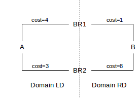
In this example, domains LD and RD join at two points. For a route across two domains joined at only a single point, the domain-local shortest paths do add up to the globally shortest path.

9.4   Loop-Free Distance Vector Algorithms

It is possible for routing-update algorithms based on the distance-vector idea to eliminate routing loops – and thus the slow-convergence problem – entirely. We present brief descriptions of two such algorithms.

9.4.1   DSDV

DSDV, or Destination-Sequenced Distance Vector, was proposed in [PB94]. It avoids routing loops by the introduction of sequence numbers: each router will always prefer routes with the most recent sequence number, and bad-news information will always have a lower sequence number then the next cycle of corrected information.

DSDV was originally proposed for MANETs (3.3.8   MANETs) and has some additional features for traffic minimization that, for simplicity, we ignore here. It is perhaps best suited for wired networks and for small, relatively stable MANETs.

DSDV forwarding tables contain entries for every other reachable node in the system. One successor of DSDV, Ad Hoc On-Demand Distance Vector routing or AODV, allows forwarding tables to contain only those destinations in active use; a mechanism is provided for discovery of routes to newly active destinations. See [PR99] and RFC 3561.

Under DSDV, each forwarding table entry contains, in addition to the destination, cost and next_hop, the current sequence number for that destination. When neighboring nodes exchange their distance-vector reachability reports, the reports include these per-destination sequence numbers.

When a router R receives a report from neighbor N for destination D, and the report contains a sequence number larger than the sequence number for D currently in R’s forwarding table, then R always updates to use the new information. The three cost-minimization rules of 9.1.1   Distance-Vector Update Rules above are used only when the incoming and existing sequence numbers are equal.

Each time a router R sends a report to its neighbors, it includes a new value for its own sequence number, which it always increments by 2. This number is then entered into each neighbor’s forwarding-table entry for R, and is then propagated throughout the network via continuing report exchanges. Any sequence number originating this way will be even, and whenever another node’s forwarding-table sequence number for R is even, then its cost for R will be finite.

Infinite-cost reports are generated in the usual way when former neighbors discover they can no longer reach one another; however, in this case each node increments the sequence number for its former neighbor by 1, thus generating an odd value. Any forwarding-table entry with infinite cost will thus always have an odd sequence number. If A and B are neighbors, and A’s current sequence number is s, and the A–B link breaks, then B will start reporting A at distance ∞ with sequence number s+1 while A will start reporting its own new sequence number s+2. Any other node now receiving a report originating with B (with sequence number s+1) will mark A as having cost ∞, but will obtain a valid route to A upon receiving a report originating from A with new (and larger) sequence number s+2.

The triggered-update mechanism is used: if a node receives a report with some destinations newly marked with infinite cost, it will in turn forward this information immediately to its other neighbors, and so on. This is, however, not essential; “bad” and “good” reports are distinguished by sequence number, not by relative arrival time.

It is now straightforward to verify that the slow-convergence problem is solved. After a link break, if there is some alternative path from router R to destination D, then R will eventually receive D’s latest even sequence number, which will be greater than any sequence number associated with any report listing D as unreachable. If, on the other hand, the break partitioned the network and there is no longer any path to D from R, then the highest sequence number circulating in R’s half of the original network will be odd and the associated table entries will all list D at cost ∞. One way or another, the network will quickly settle down to a state where every destination’s reachability is accurately described.

In fact, a stronger statement is true: not even transient routing loops are created. We outline a proof. First, whenever router R has next_hop N for a destination D, then N’s sequence number for D must be greater than or equal to R’s, as R must have obtained its current route to D from one of N’s reports. A consequence is that all routers participating in a loop for destination D must have the same (even) sequence number s for D throughout. This means that the loop would have been created if only the reports with sequence number s were circulating. As we noted in 9.1.1   Distance-Vector Update Rules, any application of the next_hop-increase rule must trace back to a broken link, and thus must involve an odd sequence number. Thus, the loop must have formed from the sequence-number-s reports by the application of the first two rules only. But this violates the claim in Exercise 10.

There is one drawback to DSDV: nodes may sometimes briefly switch to routes that are longer than optimum (though still correct). This is because a router is required to use the route with the newest sequence number, even if that route is longer than the existing route. If A and B are two neighbors of router R, and B is closer to destination D but slower to report, then every time D’s sequence number is incremented R will receive A’s longer route first, and switch to using it, and B’s shorter route shortly thereafter.

DSDV implementations usually address this by having each router R keep track of the time interval between the first arrival at R of a new route to a destination D with a given sequence number, and the arrival of the best route with that sequence number. During this interval following the arrival of the first report with a new sequence number, R will use the new route, but will refrain from including the route in the reports it sends to its neighbors, anticipating that a better route will soon arrive.

This works best when the hopcount cost metric is being used, because in this case the best route is likely to arrive first (as the news had to travel the fewest hops), and at the very least will arrive soon after the first route. However, if the network’s cost metric is unrelated to the hop count, then the time interval between first-route and best-route arrivals can involve multiple update cycles, and can be substantial.

9.4.2   EIGRP

EIGRP, or the Enhanced Interior Gateway Routing Protocol, is a once-proprietary Cisco distance-vector protocol that was released as an Internet Draft in February 2013. As with DSDV, it eliminates the risk of routing loops, even ephemeral ones. It is based on the “distributed update algorithm” (DUAL) of [JG93]. EIGRP is an actual protocol; we present here only the general algorithm. Our discussion follows [CH99].

Each router R keeps a list of neighbor routers N_R, as with any distance-vector algorithm. Each R also maintains a data structure known (somewhat misleadingly) as its topology table. It contains, for each destination D and each N in N_R, an indication of whether N has reported the ability to reach D and, if so, the reported cost c(D,N). The router also keeps, for each N in N_R, the cost c_N of the link from R to N. Finally, the forwarding-table entry for any destination can be marked “passive”, meaning safe to use, or “active”, meaning updates are in process and the route is temporarily unavailable.

Initially, we expect that for each router R and each destination D, R’s next_hop to D in its forwarding table is the neighbor N for which the following total cost is a minimum:

c(D,N) + c_N

Now suppose R receives a distance-vector report from neighbor N₁ that it can reach D with cost c(D,N₁). This is processed in the usual distance-vector way, unless it represents an increased cost and N₁ is R’s next_hop to D; this is the third case in 9.1.1   Distance-Vector Update Rules. In this case, let C be R’s current cost to D, and let us say that neighbor N of R is a feasible next_hop (feasible successor in Cisco’s terminology) if N’s cost to D (that is, c(D,N)) is strictly less than C. R then updates its route to D to use the feasible neighbor N for which c(D,N) + c_N is a minimum. Note that this may not in fact be the shortest path; it is possible that there is another neighbor M for which c(D,M)+c_M is smaller, but c(D,M)≥C. However, because N’s path to D is loop-free, and because c(D,N) < C, this new path through N must also be loop-free; this is sometimes summarized by the statement “one cannot create a loop by adopting a shorter route”.

If no neighbor N of R is feasible – which would be the case in the D—A—B example of 9.2   Distance-Vector Slow-Convergence Problem, then R invokes the “DUAL” algorithm. This is sometimes called a “diffusion” algorithm as it invokes a diffusion-like spread of table changes proceeding away from R.

Let C in this case denote the new cost from R to D as based on N₁‘s report. R marks destination D as “active” (which suppresses forwarding to D) and sends a special query to each of its neighbors, in the form of a distance-vector report indicating that its cost to D has now increased to C. The algorithm terminates when all R’s neighbors reply back with their own distance-vector reports; at that point R marks its entry for D as “passive” again.

Some neighbors may be able to process R’s report without further diffusion to other nodes, remain “passive”, and reply back to R immediately. However, other neighbors may, like R, now become “active” and continue the DUAL algorithm. In the process, R may receive other queries that elicit its distance-vector report; as long as R is “active” it will report its cost to D as C. We omit the argument that this process – and thus the network – must eventually converge.

9.5   Link-State Routing-Update Algorithm

Link-state routing is an alternative to distance-vector. It is often – though certainly not always – considered to be the routing-update algorithm class of choice for networks that are “sufficiently large”, such as those of ISPs.

In distance-vector routing, each node knows a bare minimum of network topology: it knows nothing about links beyond those to its immediate neighbors. In the link-state approach, each node keeps a maximum amount of network information: a full map of all nodes and all links. Routes are then computed locally from this map, using the shortest-path-first algorithm. The existence of this map allows, in theory, the calculation of different routes for different quality-of-service requirements. The map also allows calculation of a new route as soon as news of the failure of the existing route arrives; distance-vector protocols on the other hand must wait for news of a new route after an existing route fails.

Link-state protocols distribute network map information through a modified form of broadcast of the status of each individual link. Whenever either side of a link notices the link has died (or if a node notices that a new link has become available), it sends out link-state packets (LSPs) that “flood” the network. This broadcast process is called reliable flooding; in general broadcast protocols work poorly with networks that have even small amounts of topological looping (that is, redundant paths). Link-state protocols must ensure that every router sees every LSP, and also that no LSPs circulate repeatedly. (The acronym LSP is used by a link-state implementation known as IS-IS; the preferred acronym used by the Open Shortest Path First (OSPF) implementation is LSA, where A is for advertisement.) LSPs are sent immediately upon link-state changes, like triggered updates in distance-vector protocols except there is no “race” between “bad news” and “good news”.

It is possible for ephemeral routing loops to exist; for example, if one router has received a LSP but another has not, they may have an inconsistent view of the network and thus route to one another. However, as soon as the LSP has reached all routers involved, the loop should vanish. There are no “race conditions”, as with distance-vector routing, that can lead to persistent routing loops.

The link-state flooding algorithm avoids the usual problems of broadcast in the presence of loops by having each node keep a database of all LSP messages. The originator of each LSP includes its identity, information about the link that has changed status, and also a sequence number. Other routers need only keep in their databases the LSP packet with the largest sequence number; older LSPs can be discarded. When a router receives a LSP, it first checks its database to see if that LSP is old, or is current but has been received before; in these cases, no further action is taken. If, however, an LSP arrives with a sequence number not seen before, then in typical broadcast fashion the LSP is retransmitted over all links except the arrival interface.

As an example, consider the following arrangement of routers:

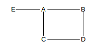
Suppose the A–E link status changes. A sends LSPs to C and B. Both these will forward the LSPs to D; suppose B’s arrives first. Then D will forward the LSP to C; the LSP traveling C→D and the LSP traveling D→C might even cross on the wire. D will ignore the second LSP copy that it receives from C and C will ignore the second copy it receives from D.

It is important that LSP sequence numbers not wrap around. (Protocols that do allow a numeric field to wrap around usually have a clear-cut idea of the “active range” that can be used to conclude that the numbering has wrapped rather than restarted; this is harder to do in the link-state context.) OSPF uses lollipop sequence-numbering here: sequence numbers begin at -2³¹ and increment to 2³¹-1. At this point they wrap around back to 0. Thus, as long as a sequence number is less than zero, it is guaranteed unique; at the same time, routing will not cease if more than 2³¹ updates are needed. Other link-state implementations use 64-bit sequence numbers.

Actual link-state implementations often give link-state records a maximum lifetime; entries must be periodically renewed.

9.5.1   Shortest-Path-First Algorithm

The next step is to compute routes from the network map, using the shortest-path-first algorithm. Here is our example network:

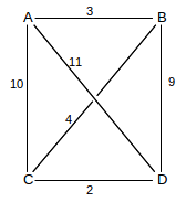
The shortest path from A to D is A-B-C-D, which has cost 3+4+2=9.

We build the set R of all shortest-path routes iteratively. Initially, R contains only the 0-length route to the start node; one new destination and route is added to R at each stage of the iteration. At each stage we have a current node, representing the node most recently added to R. The initial current node is our starting node, in this case, A.

We will also maintain a set T, for tentative, of routes to other destinations. This is also initialized to empty.

At each stage, we find all nodes which are immediate neighbors of the current node and which do not already have routes in the set R. For each such node N, we calculate the length of the route from the start node to N that goes through the current node. We see if this is our first route to N, or if the route improves on any route to N already in T; if so, we add or update the route in T accordingly.

At the end of this process, we choose the shortest path in T, and move the route and destination node to R. The destination node of this shortest path becomes the next current node. Ties can be resolved arbitrarily, but note that, as with distance-vector routing, we must choose the minimum or else the accurate-costs property will fail.

We repeat this process until all nodes have routes in the set R.

For the example above, we start with current = A and R = {⟨A,A,0⟩}. The set T will be {⟨B,B,3⟩, ⟨C,C,10⟩, ⟨D,D,11⟩}. The shortest entry is ⟨B,B,3⟩, so we move that to R and continue with current = B.

For the next stage, the neighbors of B without routes in R are C and D; the routes from A to these through B are ⟨C,B,7⟩ and ⟨D,B,12⟩. The former is an improvement on the existing T entry ⟨C,C,10⟩ and so replaces it; the latter is not an improvement over ⟨D,D,11⟩. T is now {⟨C,B,7⟩, ⟨D,D,11⟩}. The shortest route in T is that to C, so we move this node and route to R and set C to be current.

For the next stage, D is the only non-R neighbor; the path from A to D via C has entry ⟨D,B,9⟩, an improvement over the existing ⟨D,D,11⟩ in T. The only entry in T is now ⟨D,B,9⟩; this is the shortest and thus we move it to R.

We now have routes in R to all nodes, and are done.

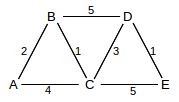
Here is another example, again with links labeled with costs:

We start with current = A. At the end of the first stage, ⟨B,B,3⟩ is moved into R, T is {⟨D,D,12⟩}, and current is B. The second stage adds ⟨C,B,5⟩ to T, and then moves this to R; current then becomes C. The third stage introduces the route (from A) ⟨D,B,10⟩; this is an improvement over ⟨D,D,12⟩ and so replaces it in T; at the end of the stage this route to D is moved to R.

A link-state source node S computes the entire path to a destination D. But as far as the actual path that a packet sent by S will take to D, S has direct control only as far as the first hop N. While the accurate-cost rule we considered in distance-vector routing will still hold, the actual path taken by the packet may differ from the path computed at the source, in the presence of alternative paths of the same length. For example, S may calculate a path S–N–A–D, and yet a packet may take path S–N–B–D, so long as the N–A–D and N–B–D paths have the same length.

Link-state routing allows calculation of routes on demand (results are then cached), or larger-scale calculation. Link-state also allows routes calculated with quality-of-service taken into account, via straightforward extension of the algorithm above.

9.6   Routing on Other Attributes

There is sometimes a desire to route on attributes other than the destination, or the destination and QoS bits. This kind of routing is decidedly nonstandard, and is generally limited to the imposition of very local routing policies. It is, however, often available.

On linux systems this is part of the Linux Advanced Routing facility, often grouped with some advanced queuing features known as Traffic Control; the combination is referred to as LARTC.

As a simple example of what can be done, suppose a site has two links L1 and L2 to the Internet, where L1 is faster and L2 serves more as a backup; in such a configuration the default route to the Internet will often be via L1. A site may wish to route some outbound traffic via L2, however, for any of the following reasons:

• the traffic may involve protocols deemed lower in priority (eg email)
• the traffic may be real-time traffic that can benefit from reduced competition on L2
• the traffic may come from lower-priority senders; eg some customers within the site may be relegated to using L2 because they are paying less

In the first two cases, routing might be based on the destination port numbers; in the third, it might be based on the source IP address.

Note that nothing can be done in the inbound direction unless L1 and L2 lead to the same ISP, and even there any special routing would be at the discretion of that ISP.

The trick with LARTC is to be compatible with existing routing-update protocols; this would be a problem if the kernel forwarding table simply added columns for other packet attributes that neighboring non-LARTC routers knew nothing about. Instead, the forwarding table is split up into multiple ⟨dest, next_hop⟩ (or ⟨dest, QoS, next_hop⟩) tables. One of these tables is the main table, and is the table that is updated by routing-update protocols interacting with neighbors. Before a packet is forwarded, administratively supplied rules are consulted to determine which table to apply; these rules are allowed to consult other packet attributes. The collection of tables and rules is known as the routing policy database.

As a simple example, in the situation above the main table would have an entry ⟨default, L1⟩ (more precisely, it would have the IP address of the far end of the L1 link instead of L1 itself). There would also be another table, perhaps named slow, with a single entry ⟨default, L2⟩. If a rule is created to have a packet routed using the “slow” table, then that packet will be forwarded via L2. Here is one such linux rule, applying to traffic from host 10.0.0.17:

``ip rule add from 10.0.0.17 table slow``

Now suppose we want to route traffic to port 25 (the SMTP port) via L2. This is harder; linux provides no support here for routing based on port numbers. However, we can instead use the iptables mechanism to “mark” all packets destined for port 25, and then create a routing-policy rule to have such marked traffic use the slow table. The mark is known as the forwarding mark, or fwmark; its value is 0 by default. The fwmark is not actually part of the packet; it is associated with the packet only while the latter remains within the kernel.

iptables --table mangle --append PREROUTING \\
         --protocol tcp --source-port 25 --jump MARK --set-mark 1

ip rule add fwmark 1 table slow

Consult the applicable man pages for further details.

The iptables mechanism can also be used to set the IP precedence bits, so that a single standard IP forwarding table can be used, though support for the IP precedence bits is limited.

9.7   Epilog

At this point we have concluded the basics of IP routing, involving routing within large (relatively) homogeneous organizations such as multi-site corporations or Internet Service Providers. Every router involved must agree to run the same protocol, and must agree to a uniform assignment of link costs.

At the very largest scales, these requirements are impractical. The next chapter is devoted to this issue of very-large-scale IP routing, eg on the global Internet.

9.8   Exercises

1. Suppose the network is as follows, where distance-vector routing update is used. Each link has cost 1, and each router has entries in its forwarding table only for its immediate neighbors (so A’s table contains ⟨B,B,1⟩, ⟨D,D,1⟩ and B’s table contains ⟨A,A,1⟩, ⟨C,C,1⟩).

A──────B──────C
│             │
│             │
D──────E──────F

(a). Suppose each node creates a report from its initial configuration and sends that to each of its neighbors. What will each node’s forwarding table be after this set of exchanges? The exchanges, in other words, are all conducted simultaneously and in parallel; no report contains new information learned by a router as part of this process.

(b). What will each node’s table be after the simultaneous-and-parallel exchange process of part (a) is repeated a second time?

Hint: you do not have to go through each exchange in detail; the only information added by an exchange is additional reachability information.

2. Now suppose the configuration of routers has the link weights shown below.

A───3───B───4───C
│               │
2               12
│               │
D───1───E───1───F

(a). As in the previous exercise, give each node’s forwarding table after each node exchanges with its immediate neighbors simultaneously and in parallel.

(b). How many iterations of such parallel exchanges will it take before C learns to reach F via B; that is, before it creates the entry ⟨F,B,11⟩?

3. Suppose a router R has the following distance-vector table:

destination	cost	next hop
A	5	R1
B	6	R1
C	7	R2
D	8	R2
E	9	R3

R now receives the following report from R1; the cost of the R–R1 link is 1.

destination	cost
A	4
B	7
C	7
D	6
E	8
F	8

Give R’s updated table after it processes R1’s report. For each entry that changes, give a brief explanation, in the style of 9.1.5   Example 4.

4. Suppose nodes A, B, C, D, E and F form a network in which all links have cost 1. The forwarding tables for A and F are as follows:

A’s table

destination	cost	next hop
B	1	B
C	1	C
D	2	B
E	2	C
F	3	B

F’s table

destination	cost	next hop
A	3	D
B	2	D
C	2	E
D	1	D
E	1	E

These tables imply that A is directly connected only to B and C, and that F is directly connected only to D and E, because these are the only destinations reachable with a cost of 1. Give all other direct connections that must exist, and draw the network.

5. Suppose A, B, C, D and E are connected as follows. Each link has cost 1, and so each forwarding table is uniquely determined; B’s table is ⟨A,A,1⟩, ⟨C,C,1⟩, ⟨D,A,2⟩, ⟨E,C,2⟩. Distance-vector routing update is used.

Now suppose the D–E link fails, and so D updates its entry for E to ⟨E,-,∞⟩.

(a). Give A’s table after D reports ⟨E,∞⟩ to A

(b). Give B’s table after A reports to B

(c). Give A’s table after B reports to A; note that B has an entry ⟨E,C,2⟩

(d). Give D’s table after A reports to D.

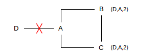
6. Consider the network in 9.2.1.1   Split Horizon:, using distance-vector routing updates.

      ┌───────B  ⟨D,A,2⟩
      │       │
D──x──A       │
      │       │
      └───────C  ⟨D,A,2⟩

Suppose the D–A link breaks and then

• A reports ⟨D,∞⟩ to B (as before)
• C reports ⟨D,2⟩ to B (as before)
• A now reports ⟨D,∞⟩ to C (instead of B reporting ⟨D,3⟩ to A)

(a). What report will lead to the formation of the routing loop?

(b). What report will eliminate the possibility of the routing loop?

7. Suppose the network of 9.2   Distance-Vector Slow-Convergence Problem is changed to the following. Distance-vector update is used; again, the A–D link breaks.

          ⟨D,D,1⟩       ⟨D,E,2⟩
D───────────A───────────B
│                       │
│                       │
└───────────────────────E

(a). Explain why B’s report back to A, after A reports ⟨D,-,∞⟩, is now valid.

(b). Explain why hold down (9.2.1.3   Hold Down) will delay the use of the new route A–B–E–D.

8. Suppose the routers are A, B, C, D, E and F, and all link costs are 1. The distance-vector forwarding tables for A and F are below. Give the network with the fewest links that is consistent with these tables. Hint: any destination reached at cost 1 is directly connected; if X reaches Y via Z at cost 2, then Z and Y must be directly connected.

A’s table

dest	cost	next_hop
B	1	B
C	1	C
D	2	C
E	2	C
F	3	B

F’s table

dest	cost	next_hop
A	3	E
B	2	D
C	2	D
D	1	D
E	1	E

9. (a) Suppose routers A and B somehow end up with respective forwarding-table entries ⟨D,B,n⟩ and ⟨D,A,m⟩, thus creating a routing loop. Explain why the loop may be removed more quickly if A and B both use poison reverse with split horizon, versus if A and B use split horizon only.

(b). Suppose the network looks like the following. The A–B link is extremely slow.

A────────────┐
│            │
│            C─────────D
│            │
B────────────┘

Suppose A and B send reports to each other advertising their routes to D, and immediately afterwards the C–D link breaks and C reports to A and B that D is unreachable. After those unreachability reports are processed, A and B’s reports sent to each other before the break finally arrive. Explain why the network is now in the state described in part (a).

10. Suppose the distance-vector algorithm is run on a network and no links break (so by the last paragraph of 9.1.1   Distance-Vector Update Rules the next_hop-increase rule is never applied).

(a). Prove that whenever A is B’s next_hop to destination D, then A’s cost to D is strictly less than B’s. Hint: assume that if this claim is true, then it remains true after any application of the rules in 9.1.1   Distance-Vector Update Rules. If the lower-cost rule is applied to B after receiving a report from A, resulting in a change to B’s cost to D, then one needs to show A’s cost is less than B’s, and also B’s new cost is less than that of any neighbor C that uses B as its next_hop to D.

(b). Use (a) to prove that no routing loops ever form.

11. Give a scenario illustrating how a (very temporary!) routing loop might form in link-state routing.

12. Use the Shortest Path First algorithm to find the shortest path from A to E in the network below. Show the sets R and T, and the node current, after each step.

13. Suppose you take a laptop, plug it into an Ethernet LAN, and connect to the same LAN via Wi-Fi. From laptop to LAN there are now two routes. Which route will be preferred? How can you tell which way traffic is flowing? How can you configure your OS to prefer one path or another?