10   Large-Scale IP Routing

In the previous chapter we considered two classes of routing-update algorithms: distance-vector and link-state. Each of these approaches requires that participating routers have agreed not just to a common protocol, but also to a common understanding of how link costs are to be assigned. We will address this further below in 10.6   Border Gateway Protocol, BGP, but the basic problem is that if one site prefers the hop-count approach, assigning every link a cost of 1, while another site prefers to assign link costs in proportion to their bandwidth, then path cost comparisons between the two sites simply cannot be done. In general, we cannot even “translate” costs from one site to another, because the paths themselves depend on the cost assignment strategy.

The term routing domain is used to refer to a set of routers under common administration, using a common link-cost assignment. Another term for this is autonomous system. While use of a common routing-update protocol within the routing domain is not an absolute requirement – for example, some subnets may internally use distance-vector while the site’s “backbone” routers use link-state – we can assume that all routers have a uniform view of the site’s topology and cost metrics.

One of the things included in the term “large-scale” IP routing is the coordination of routing between multiple routing domains. Even in the earliest Internet there were multiple routing domains, if for no other reason than that how to measure link costs was (and still is) too unsettled to set in stone. However, another component of large-scale routing is support for hierarchical routing, above the level of subnets; we turn to this next.

10.1   Classless Internet Domain Routing: CIDR

CIDR is the mechanism for supporting hierarchical routing in the Internet backbone. Subnetting moves the network/host division line further rightwards; CIDR allows moving it to the left as well. With subnetting, the revised division line is visible only within the organization that owns the IP network address; subnetting is not visible outside. CIDR allows aggregation of IP address blocks in a way that is visible to the Internet backbone.

When CIDR was introduced in 1993, the following were some of the justifications for it, all relating to the increasing size of the backbone IP forwarding tables, and expressed in terms of the then-current Class A/B/C mechanism:

• The Internet is running out of Class B addresses (this happened in the mid-1990’s)
• There are too many Class C’s (the most numerous) for backbone forwarding tables to be efficient
• Eventually IANA (the Internet Assigned Numbers Authority) will run out of IP addresses (this happened in 2011)

Assigning non-CIDRed multiple Class C’s in lieu of a single Class B would have helped with the first point in the list above, but made the second point worse.

Ironically, the current (2013) very tight market for IP address blocks is likely to lead to larger and larger backbone IP forwarding tables, as sites are forced to use multiple small address blocks instead of one large block.

By the year 2000, CIDR had essentially eliminated the Class A/B/C mechanism from the backbone Internet, and had more-or-less completely changed how backbone routing worked. You purchased an address block from a provider or some other IP address allocator, and it could be whatever size you needed, from /27 to /15.

What CIDR enabled is IP routing based on an address prefix of any length; the Class A/B/C mechanism of course used fixed prefix lengths of 8, 16 and 24 bits. Furthermore, CIDR allows different routers, at different levels of the backbone, to route on prefixes of different lengths.

CIDR was formally introduced by RFC 1518 and RFC 1519. For a while there were strategies in place to support compatibility with non-CIDR-aware routers; these are now obsolete. In particular, it is no longer appropriate for large-scale routers to fall back on the Class A/B/C mechanism in the absence of CIDR information; if the latter is missing, the routing should fail.

The basic strategy of CIDR is to consolidate multiple networks going to the same destination into a single entry. Suppose a router has four class C’s all to the same destination:

200.7.0.0/24 ⟶ foo

200.7.1.0/24 ⟶ foo

200.7.2.0/24 ⟶ foo

200.7.3.0/24 ⟶ foo

The router can replace all these with the single entry

200.7.0.0/22 ⟶ foo

It does not matter here if foo represents a single ultimate destination or if it represents four sites that just happen to be routed to the same next_hop.

It is worth looking closely at the arithmetic to see why the single entry uses /22. This means that the first 22 bits must match 200.7.0.0; this is all of the first and second bytes and the first six bits of the third byte. Let us look at the third byte of the network addresses above in binary:

200.7.000000 00.0/24 ⟶ foo

200.7.000000 01.0/24 ⟶ foo

200.7.000000 10.0/24 ⟶ foo

200.7.000000 11.0/24 ⟶ foo

The /24 means that the network addresses stop at the end of the third byte. The four entries above cover every possible combination of the last two bits of the third byte; for an address to match one of the entries above it suffices to begin 200.7 and then to have 0-bits as the first six bits of the third byte. This is another way of saying the address must match 200.7.0.0/22.

Most implementations actually use a bitmask, eg FF.FF.FC.00 (in hex) rather than the number 22; note 0xFC = 1111 1100 with 6 leading 1-bits, so FF.FF.FC.00 has 8+8+6=22 1-bits followed by 10 0-bits.

The IP delivery algorithm of 7.5   The Classless IP Delivery Algorithm still works with CIDR, with the understanding that the router’s forwarding table can now have a network-prefix length associated with any entry. Given a destination D, we search the forwarding table for network-prefix destinations B/k until we find a match; that is, equality of the first k bits. In terms of masks, given a destination D and a list of table entries ⟨prefix,mask⟩ = ⟨B[i],M[i]⟩, we search for i such that (D & M[i]) = B[i].

It is possible to have multiple matches, and responsibility for avoiding this is much too distributed to be declared illegal by IETF mandate. Instead, CIDR introduced the longest-match rule: if destination D matches both B₁/k₁ and B₂/k₂, with k₁ < k₂, then the longer match B₂/k₂ match is to be used. (Note that if D matches two distinct entries B₁/k₁ and B₂/k₂ then either k₁ < k₂ or k₂ < k₁).

10.2   Hierarchical Routing

Strictly speaking, CIDR is simply a mechanism for routing to IP address blocks of any prefix length; that is, for setting the network/host division point to an arbitrary place within the 32-bit IP address.

However, by making this network/host division point variable, CIDR introduced support for routing on different prefix lengths at different places in the backbone routing infrastructure. For example, top-level routers might route on /8 or /9 prefixes, while intermediate routers might route based on prefixes of length 14. This feature of routing on fewer bits at one point in the Internet and more bits at another point is exactly what is meant by hierarchical routing.

We earlier saw hierarchical routing in the context of subnets: traffic might first be routed to a class-B site 147.126.0.0/16, and then, within that site, to subnets such as 147.126.1.0/24, 147.126.2.0/24, etc. But with CIDR the hierarchy can be much more flexible: the top level of the hierarchy can be much larger than the “customer” level, lower levels need not be administratively controlled by the higher levels (as is the case with subnets), and more than two levels can be used.

CIDR is an address-block-allocation mechanism; it does not directly speak to the kinds of policy we might wish to implement with it. Here are three possible applications; the latter two involve hierarchical routing:

• Application 1 (legacy): CIDR allows IANA to allocate multiple blocks of Class C, or fragments of a Class A, to a single customer, so as to require only a single forwarding-table entry
• Application 2 (legacy): CIDR allows opportunistic aggregation of routes: a router that sees the four 200.7.x.0/24 routes above in its table may consolidate them into a single entry.
• Application 3 (current): CIDR allows huge provider blocks, with suballocation by the provider. This is known as provider-based routing.
• Application 4 (hypothetical): CIDR allows huge regional blocks, with suballocation within the region, somewhat like the original scheme for US phone numbers with area codes. This is known as geographical routing.

Hierarchical routing does introduce one new wrinkle: the routes chosen may no longer be globally optimal. Suppose, for example, we are trying to route to prefix 200.20.0.0/16. Suppose at the top level that traffic to 200.0.0.0/8 is routed to router R1, and R1 then routes traffic to 200.20.0.0/16 to R2. A packet sent to 200.20.1.2 by an independent router R3 would always pass through R1, even if there were a shorter path R3→R4→R2 that bypassed R1. This is addressed in further detail below in 10.4.3   Provider-Based Hierarchical Routing.

We can avoid this by declaring that CIDR will only be used when it turns out that, in the language of the example of the preceding paragraph, the best path to reach 200.20.0.0/16 is always through R1. But this is seldom the case, and is even less likely to remain the case as new links are added. Such a policy also defeats much of the potential benefit of CIDR at reducing router forwarding-table size by supporting the creation of arbitrary-sized address blocks and then routing to them as a single unit. The Internet backbone might be much happier if all routers simply had to maintain a single entry ⟨200.0.0.0/8, R1⟩, versus 256 entries ⟨200.x.0.0/16, R1⟩ for all but one value of x.

10.3   Legacy Routing

Back in the days of NSFNet, the Internet backbone was a single routing domain. While most customers did not connect directly to the backbone, the intervening providers tended to be relatively compact, geographically – that is, regional – and often had a single primary routing-exchange point with the backbone. IP addresses were allocated to subscribers directly by the IANA, and the backbone forwarding tables contained entries for every site, even the Class C’s.

Because the NSFNet backbone and the regional providers did not necessarily share link-cost information, routes were even at this early point not necessarily globally optimal; compromises and approximations were made. However, in the NSFNet model routers generally did find a reasonable approximation to the shortest path to each site referenced by the backbone tables. While the legacy backbone routing domain was not all-encompassing, if there were differences between two routes, at least the backbone portions – the longest components – would be identical.

10.4   Provider-Based Routing

In provider-based routing, large CIDR blocks are allocated to large-scale providers. The different providers each know how to route to one another. Subscribers (usually) obtain their IP addresses from within their providers’ blocks; thus, traffic from the outside is routed first to the provider, and then, within the provider’s routing domain, to the subscriber. We may even have a hierarchy of providers, so packets would be routed first to the large-scale provider, and eventually to the local provider. There may no longer be a central backbone; instead, multiple providers may each build parallel transcontinental networks.

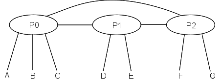
Here is a simpler example, in which providers have unique paths to one another. Suppose we have providers P0, P1 and P2, with customers as follows:

• P0: customers A,B,C
• P1: customers D,E
• P2: customers F,G

We will also assume that each provider has an IP address block as follows:

• P0: 200.0.0.0/8
• P1: 201.0.0.0/8
• P2: 202.0.0.0/8

Let us now allocate addresses to the customers:

A: 200.0.0.0/16

B: 200.1.0.0/16

C: 200.2.16.0/20 (16 = 0001 0000)

D: 201.0.0.0/16

E: 201.1.0.0/16

F: 202.0.0.0/16

G: 202.1.0.0/16

The routing model is that packets are first routed to the appropriate provider, and then to the customer. While this model may not in general guarantee the shortest end-to-end path, it does in this case because each provider has a single point of interconnection to the others. Here is the network diagram:

With this diagram, P0’s forwarding table looks something like this:

destination	next_hop
200.0.0.0/16	A
200.1.0.0/16	B
200.2.16.0/20	C
201.0.0.0/8	P1
202.0.0.0/8	P2

That is, P0’s table consists of

• one entry for each of P0’s own customers
• one entry for each other provider

If we had 1,000,000 customers divided equally among 100 providers, then each provider’s table would have only 10,099 entries: 10,000 for its own customers and 99 for the other providers. Without CIDR, each provider’s forwarding table would have 1,000,000 entries.

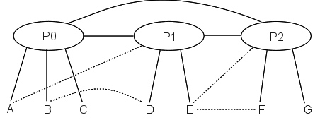
Even if we have some additional “secondary” links, that is, additional links that do not create alternative paths between providers, the routing remains relatively straightforward. Shown here are the private customer-to-customer links C–D and E–F; these are likely used only by the customers they connect. Two customers are multi-homed; that is, they have connections to alternative providers: A–P1 and E–P2. Typically, though, while A and E may use these secondary links all they want for outbound traffic, their respective inbound traffic would still go through their primary providers P0 and P1 respectively.

10.4.1   Internet Exchange Points

The long links joining providers in these diagrams are somewhat misleading; providers do not always like sharing long links and the attendant problems of sharing responsibility for failures. Instead, providers often connect to one another at Internet eXchange Points or IXPs; the link P0──────P1 might actually be P0───IXP───P1, where P0 owns the left-hand link and P1 the right-hand. IXPs can either be third-party sites open to all providers, or private exchange points. The term “Metropolitan Area Exchange”, or MAE, appears in the names of the IXPs MAE-East, originally near Washington DC, and MAE-West, originally in San Jose, California; each of these is now actually a set of IXPs. MAE in this context is now a trademark.

10.4.2   CIDR and Staying Out of Jail

Suppose we want to change providers. One way we can do this is to accept a new IP-address block from the new provider, and change all our IP addresses. The paper Renumbering: Threat or Menace [LKCT96] was frequently cited – at least in the early days of CIDR – as an intimation that such renumbering was inevitably a Bad Thing. In principle, therefore, we would like to allow at least the option of keeping our IP address allocation while changing providers.

An address-allocation standard that did not allow changing of providers might even be a violation of the US Sherman Antitrust Act; see American Society of Mechanical Engineers v Hydrolevel Corporation, 456 US 556 (1982). The IETF thus had the added incentive of wanting to stay out of jail, when writing the CIDR standard so as to allow portability between providers (actually, antitrust violations usually involve civil penalties).

The CIDR longest-match rule turns out to be exactly what we (and the IETF) need. Suppose, in the diagrams above, that customer C wants to move from P0 to P1, and does not want to renumber. What routing changes need to be made? One solution is for P0 to add a route ⟨200.2.16.0/20, P1⟩ that routes all of C’s traffic to P1; P1 will then forward that traffic on to C. P1’s table will be as follows, and P1 will use the longest-match rule to distinguish traffic for its new customer C from traffic bound for P0.

destination	next_hop
200.0.0.0/8	P0
202.0.0.0/8	P2
201.0.0.0/16	D
201.1.0.0/16	E
200.2.16.0/20	C

This does work, but all C’s inbound traffic except for that originating in P1 will now be routed through C’s ex-provider P0, which as an ex-provider may not be on the best of terms with C. Also, the routing is inefficient: C’s traffic from P2 is routed P2→P0→P1 instead of the more direct P2→P1.

A better solution is for all providers other than P1 to add the route ⟨200.2.16.0/20, P1⟩. While traffic to 200.0.0.0/8 otherwise goes to P0, this particular sub-block is instead routed by each provider to P1. The important case here is P2, as a stand-in for all other providers and their routers: P2 routes 200.0.0.0/8 traffic to P0 except for the block 200.2.16.0/20, which goes to P1.

Having every other provider in the world need to add an entry for C is going to cost some money, and, one way or another, C will be the one to pay. But at least there is a choice: C can consent to renumbering (which is not difficult if they have been diligent in using DHCP and perhaps NAT too), or they can pay to keep their old address block.

As for the second diagram above, with the various private links (shown as dashed lines), it is likely that the longest-match rule is not needed for these links to work. A’s “private” link to P1 might only mean that

• A can send outbound traffic via P1
• P1 forwards A’s traffic to A via the private link

P2, in other words, is still free to route to A via P0. P1 may not advertise its route to A to anyone else.

10.4.3   Provider-Based Hierarchical Routing

With provider-based routing, the route taken may no longer be end-to-end optimal; we have replaced the problem of finding an optimal route from A to B with the two problems of finding an optimal route from A to B’s provider, and then from that provider entry point to B; the second strategy may not yield the same result. This second strategy mirrors the two-step routing process of first routing on the address bits that identify the provider, and then routing on the address bits including the subscriber portion.

Consider the following example, in which providers P1 and P2 have three interconnection links (r1–s1, r2–s2 and r3–s3), each with cost 1. We assume that P1’s costs happen to be comparable with P2’s costs.

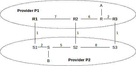
The globally shortest path between A and B is via the r2–s2 crossover, with total length 5+1+5=11. However, traffic from A to B will be routed by P1 to its closest crossover to P2, namely the r3–s3 link. The total path is 2+1+8+5=16. Traffic from B to A will be routed by P2 via the r1–s1 crossover, for a length of 2+1+7+6=16. This routing strategy is sometimes called hot-potato routing; each provider tries to get rid of any traffic (the potatoes) as quickly as possible, by routing to the closest exit point.

Not only are the paths taken inefficient, but the A⟶B and B⟶A paths are now asymmetric. This can be a problem if forward and reverse timings are critical, or if one of P1 or P2 has significantly more bandwidth or less congestion than the other. In practice, however, route asymmetry is of little consequence.

As for the route inefficiency itself, this also is not necessarily a significant problem; the primary reason routing-update algorithms focus on the shortest path is to guarantee that all computed paths are loop-free. As long as each half of a path is loop-free, and the halves do not intersect except at their common midpoint, these paths too will be loop-free.

The BGP “MED” value (10.6.5.3   MULTI_EXIT_DISC) offers an optional mechanism for P1 to agree that A⟶B traffic should take the r1–s1 crossover. This might be desired if P1’s network were “better” and customer A was willing to pay extra to keep its traffic within P1’s network as long as possible.

10.5   Geographical Routing

The classical alternative to provider-based routing is geographical routing; the archetypal model for this is the telephone area code system. A call from anywhere in the US to Loyola University’s main switchboard, 773-274-3000, would traditionally be routed first to the 773 area code in Chicago. From there the call would be routed to the north-side 274 exchange, and from there to subscriber 3000. A similar strategy can be used for IP routing.

Geographical addressing has some advantages. Figuring out a good route to a destination is usually straightforward, and close to optimal in terms of the path physical distance. Changing providers never involves renumbering (though moving may). And approximate IP address geolocation (determining a host’s location from its IP address) is automatic.

Geographical routing has some minor technical problems. First, routing may be inefficient between immediate neighbors A and B that happen to be split by a boundary for larger geographical areas; the path might go from A to the center of A’s region to the center of B’s region and then to B. Another problem is that some larger sites (eg large corporations) are themselves geographically distributed; if efficiency is the goal, each office of such a site would need a separate IP address block appropriate for its physical location.

But the real issue with geographical routing is apparently the business question of who carries the traffic. The provider-based model has a very natural answer to this: every link is owned by a specific provider. For geographical IP routing, my local provider might know at once from the prefix that a packet of mine is to be delivered from Chicago to San Francisco, but who will carry it there? My provider might have to enter into different traffic contracts for multiple different regions. If different local providers make different arrangements for long-haul packet delivery, the routing efficiency (at least in terms of table size) of geographical routing is likely lost. Finally, there is no natural answer for who should own those long inter-region links. It may be useful to recall that the present area-code system was created when the US telephone system was an AT&T monopoly, and the question of who carried traffic did not exist.

That said, the top five Regional Internet Registries represent geographical regions (usually continents), and provider-based addressing is below that level. That is, the IANA handed out address blocks to the geographical RIRs, and the RIRs then allocated address blocks to providers.

At the intercontinental level, geography does matter: some physical link paths are genuinely more expensive than other (shorter) paths. It is much easier to string terrestrial cable than undersea cable. However, within a continent physical distance does not always matter as much as might be supposed. Furthermore, a large geographically spread-out provider can always divide up its address blocks by region, allowing internal geographical routing to the correct region.

Here is a picture of IP address allocation as of 2006: http://xkcd.com/195.

10.6   Border Gateway Protocol, BGP

In 9   Routing-Update Algorithms, we considered interior routing-update protocols. For both Distance-Vector and Link State methods, the per-link cost played an essential role: by trying to minimize the cost, we were assured that no routing loops would be present in a stable network.

But when systems under different administration (eg two large ISPs) talk to each other, comparing metrics simply does not work. Each side’s metrics may be based on any of the following:

• hopcount
• bandwidth
• cost
• congestion

One provider’s metric may even use larger numbers for better routes (though if this is done then total path costs, or preference, cannot be obtained simply by adding the per-link values). Any attempt at comparison of values from the different sides is a comparison of apples and oranges.

The Border Gateway Protocol, or BGP, is assigned the job of handling exchange of routing information between neighboring independent organizations; this is sometimes called exterior routing. The current version is BGP-4, documented in RFC 4271. The BGP term for a routing domain under coordinated administration, and using one consistent link-cost metric throughout, is Autonomous System, or AS. That said, all that is strictly required is that all BGP routers within an AS have the same consistent view of routing, and in fact some Autonomous Systems do run multiple routing protocols and may even use different metrics at different points. As indicated above, BGP does not support the exchange of link-cost information between Autonomous Systems.

BGP also has a second goal, in addition to the purely technical problem of finding routes in the absence of cost information: BGP also provides support for policy-based routing; that is, for making routing decisions based on managerial or administrative input (perhaps regarding who is paying what for the traffic carried).

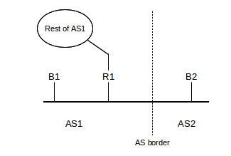
Every non-leaf site (and some large leaf sites) has one or more BGP speakers: the routers that run BGP. If there is more than one, they must remain coordinated with one another so as to present a consistent view of the site’s connections and advertisements; this coordination process is sometimes called internal BGP to distinguish it from the communication with neighboring Autonomous Systems. The latter process is then known as external BGP.

The BGP speakers of a site are often not the busy border routers that connect directly to the neighboring AS, though they are usually located near them and are often on the same subnet. Each interconnection point with a neighboring AS generally needs its own BGP speaker. Connections between BGP speakers of neighboring Autonomous Systems – sometimes called BGP peers – are generally configured administratively; they are not subject to a “neighbor discovery” process like that used by most interior routers.

The BGP speakers must maintain a database of all routes received, not just of the routes actually used. However, the speakers exchange with neighbors only the routes they (and thus their AS) use themselves; this is a firm BGP rule.

The current BGP standard is RFC 4271.

10.6.1   AS-paths

At its most basic level, BGP involves the exchange of lists of reachable destinations, like distance-vector routing without the distance information. But that strategy, alone, cannot avoid routing loops. BGP solves the loop problem by having routers exchange, not just destination information, but also the entire path used to reach each destination. Paths including each router would be too cumbersome; instead, BGP abbreviates the path to the list of AS’s traversed; this is called the AS-path. This allows routers to make sure their routes do not traverse any AS more than once, and thus do not have loops.

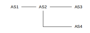
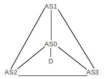
As an example of this, consider the network below, in which we consider Autonomous Systems also to be destinations. Initially, we will assume that each AS discovers its immediate neighbors. AS3 and AS5 will then each advertise to AS4 their routes to AS2, but AS4 will have no reason at this level to prefer one route to the other (BGP does use the shortest AS-path as part of its tie-breaking rule, but, before falling back on that rule, AS4 is likely to have a commercial preference for which of AS3 and AS5 it uses to reach AS2).

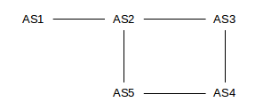
Also, AS2 will advertise to AS3 its route to reach AS1; that advertisement will contain the AS-path ⟨AS2,AS1⟩. Similarly, AS3 will advertise this route to AS4 and then AS4 will advertise it to AS5. When AS5 in turn advertises this AS1-route to AS2, it will include the entire AS-path ⟨AS5,AS4,AS3,AS2,AS1⟩, and AS2 would know not to use this route because it would see that it is a member of the AS-path. Thus, BGP is spared the kind of slow-convergence problem that traditional distance-vector approaches were subject to.

It is theoretically possible that the shortest path (in the sense, say, of the hopcount metric) from one host to another traverses some AS twice. If so, BGP will not allow this route.

AS-paths potentially add considerably to the size of the AS database. The number of paths a site must keep track of is proportional to the number of AS’s, because there will be one AS-path to each destination AS. (Actually, an AS may have to record many times that many AS-paths, as an AS may hear of AS-paths that it elects not to use.) Typically there are several thousand AS’s in the world. Let A be the number of AS’s. Typically the average length of an AS-path is about log(A), although this depends on connectivity. The amount of memory required by BGP is

C×A×log(A) + K×N,

where C and K are constants.

The other major goal of BGP is to allow some degree of administrative input to what, for interior routing, is largely a technical calculation (though an interior-routing administrator can set link costs). BGP is the interface between large ISPs, and can be used to implement contractual agreements made regarding which ISPs will carry other ISPs’ traffic. If ISP2 tells ISP1 it has a good route to destination D, but ISP1 chooses not to send traffic to ISP2, BGP can be used to implement this.

Despite the exchange of AS-path information, temporary routing loops may still exist. This is because BGP may first decide to use a route and only then export the new AS-path; the AS on the other side may realize there is a problem as soon as the AS-path is received but by then the loop will have at least briefly been in existence. See the first example below in 10.6.8   Examples of BGP Instability.

BGP’s predecessor was EGP, which guaranteed loop-free routes by allowing only a single route to any AS, thus forcing the Internet into a tree topology, at least at the level of Autonomous Systems. The AS graph could contain no cycles or alternative routes, and hence there could be no redundancy provided by alternative paths. EGP also thus avoided having to make decisions as to the preferred path; there was never more than one choice. EGP was sometimes described as a reachability protocol; its only concern was whether a given network was reachable.

10.6.2   AS-Paths and Route Aggregation

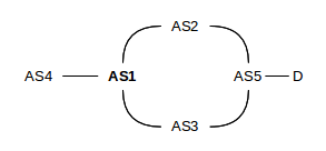
There is some conflict between the goal of reporting precise AS-paths to each destination, and of consolidating as many address prefixes as possible into a single prefix (single CIDR block). Consider the following network:

Suppose AS2 has paths

path=⟨AS2⟩, destination 200.0.0/23

path=⟨AS2,AS3⟩, destination 200.0.2/24

path=⟨AS2,AS4⟩, destination 200.0.3/24

If AS2 wants to optimize address-block aggregation using CIDR, it may prefer to aggregate the three destinations into the single block 200.0.0/22. In this case there would be two options for how AS2 reports its routes to AS1:

• Option 1: report 200.0.0/22 with path ⟨AS2⟩. But this ignores the AS’s AS3 and AS4! These are legitimately part of the AS-paths to some of the destinations within the block 200.0.0/22; loop detection could conceivably now fail.
• Option 2: report 200.0.0/22 with path ⟨AS2,AS3,AS4⟩, which is not a real path but which does include all the AS’s involved. This ensures that the loop-detection algorithm works, but artificially inflates the length of the AS-path, which is used for certain tie-breaking decisions.

As neither of these options is desirable, the concept of the AS-set was introduced. A list of Autonomous Systems traversed in order now becomes an AS-sequence. In the example above, AS2 can thus report net 200.0.0/22 with

• AS-sequence=⟨AS2⟩
• AS-set={AS3,AS4}

AS2 thus both achieves the desired aggregation and also accurately reports the AS-path length.

The AS-path can in general be an arbitrary list of AS-sequence and AS-set parts, but in cases of simple aggregation such as the example here, there will be one AS-sequence followed by one AS-set.

RFC 6472 now recommends against using AS-sets entirely, and recommends that aggregation as above be avoided.

10.6.3   Transit Traffic

It is helpful to distinguish between two kinds of traffic, as seen from a given AS. Local traffic is traffic that either originates or terminates at that AS; this is traffic that “belongs” to that AS. At leaf sites (that is, sites that connect only to their ISP and not to other sites), all traffic is local.

The other kind of traffic is transit traffic; the AS is forwarding it along on behalf of some nonlocal party. For ISPs, most traffic is transit traffic. A large almost-leaf site might also carry a small amount of transit traffic for one particular related (but autonomous!) organization.

The decision as to whether to carry transit traffic is a classic example of an administrative choice, implemented by BGP’s support for policy-based routing.

10.6.4   BGP Filtering and Policy Routing

As stated above, one of the goals of BGP is to support policy routing; that is, routing based on managerial or administrative concerns in addition to technical ones. A BGP speaker may be aware of multiple routes to a destination. To choose the one route that we will use, it may combine a mixture of optimization rules and policy rules. Some examples of policy rules might be:

• do not use AS13 as we have an adversarial relationship with them
• do not allow transit traffic

BGP implements policy through filtering rules – that is, rules that allow rejection of certain routes – at three different stages:

1. Import filtering is applied to the lists of routes a BGP speaker receives from its neighbors.
2. Best-path selection is then applied as that BGP speaker chooses which of the routes accepted by the first step it will actually use.
3. Export filtering is done to decide what routes from the previous step a BGP speaker will actually advertise. A BGP speaker can only advertise paths it uses, but does not have to advertise every such path.

While there are standard default rules for all these (accept everything imported, use simple tie-breakers, export everything), a site will usually implement at least some policy rules through this filtering process (eg “prefer routes through the ISP we have a contract with”).

As an example of import filtering, a site might elect to ignore all routes from a particular neighbor, or to ignore all routes whose AS-path contains a particular AS, or to ignore temporarily all routes from a neighbor that has demonstrated too much recent “route instability” (that is, rapidly changing routes). Import filtering can also be done in the best-path-selection stage. Finally, while it is not commonly useful, import filtering can involve rather strange criteria; for example, in 10.6.8   Examples of BGP Instability we will consider examples where AS1 prefers routes with AS-path ⟨AS3,AS2⟩ to the strictly shorter path ⟨AS2⟩.

The next stage is best-path selection, for which the first step is to eliminate AS-paths with loops. Even if the neighbors have been diligent in not advertising paths with loops, an AS will still need to reject routes that contain itself in the associated AS-path.

The next step in the best-path-selection stage, generally the most important in BGP configuration, is to assign a local_preference, or weight, to each route received. An AS may have policies that add a certain amount to the local_preference for routes that use a certain AS, etc. Very commonly, larger sites will have preferences based on contractual arrangements with particular neighbors. Provider AS’s, for example, will in general prefer routes that go through their customers, as these are “cheaper”. A smaller ISP that connects to two or more larger ones might be paying to route almost all its outbound traffic through a particular one of the two; its local_preference values will then implement this choice. After BGP calculates the local_preference value for every route, the routes with the best local_preference are then selected.

Domains are free to choose their local_preference rules however they wish. Some choices may lead to instability, below, so domains are encouraged to set their rules in accordance with some standard principles, also below.

In the event of ties – two routes to the same destination with the same local_preference – a first tie-breaker rule is to prefer the route with the shorter AS-path. While this superficially resembles a shortest-path algorithm, the real work should have been done in administratively assigning local_preference values.

Local_preference values are communicated internally via the LOCAL_PREF path attribute, below. They are not shared with other Autonomous Systems.

The final significant step of the route-selection phase is to apply the Multi_Exit_Discriminator value; we postpone this until below. A site may very well choose to ignore this value entirely. There may then be additional trivial tie-breaker rules; note that if a tie-breaker rule assigns significant traffic to one AS over another, then it may have significant economic consequences and shouldn’t be considered “trivial”. If this situation is detected, it would probably be addressed in the local-preferences phase.

After the best-path-selection stage is complete, the BGP speaker has now selected the routes it will use. The final stage is to decide what rules will be exported to which neighbors. Only routes the BGP speaker will use – that is, routes that have made it to this point – can be exported; a site cannot route to destination D through AS1 but export a route claiming D can be reached through AS2.

It is at the export-filtering stage that an AS can enforce no-transit rules. If it does not wish to carry transit traffic to destination D, it will not advertise D to any of its AS-neighbors.

The export stage can lead to anomalies. Suppose, for example, that AS1 reaches D and AS5 via AS2, and announces this to AS4.

Later AS1 switches to reaching D via AS3, but A is forbidden by policy to announce AS3-paths to AS4. Then A must simply withdraw the announcement to AS4 that it could reach D at all, even though the route to D via AS2 is still there.

10.6.5   BGP Path attributes

BGP supports the inclusion of various path attributes when exchanging routing information. Attributes exchanged with neighbors can be transitive or non-transitive; the difference is that if a neighbor AS does not recognize a received path attribute then it should pass it along anyway if it is marked transitive, but not otherwise. Some path attributes are entirely local, that is, internal to the AS of origin. Other flags are used to indicate whether recognition of a path attribute is required or optional, and whether recognition can be partial or must be complete.

The AS-path itself is perhaps the most fundamental path attribute. Here are a few other common attributes:

10.6.5.1   NEXT_HOP

This mandatory external attribute allows BGP speaker B1 of AS1 to inform its BGP peer B2 of AS2 what actual router to use to reach a given destination. If B1, B2 and AS1’s actual border router R1 are all on the same subnet, B1 will include R1’s IP address as its NEXT_HOP attribute. If B1 is not on the same subnet as B2, it may not know R1’s IP address; in this case it may include its own IP address as the NEXT_HOP attribute. Routers on AS2’s side will then look up the “immediate next hop” they would use as the first step to reach B1, and forward traffic there. This should either be R1 or should lead to R1, which will then route the traffic properly (not necessarily on to B1).

10.6.5.2   LOCAL_PREF

If one BGP speaker in an AS has been configured with local_preference values, used in the best-path-selection phase above, it uses the LOCAL_PREF path attribute to share those preferences with all other BGP speakers at a site.

10.6.5.3   MULTI_EXIT_DISC

The Multi-Exit Discriminator, or MED, attribute allows one AS to learn something of the internal structure of another AS, should it elect to do so. Using the MED information provided by a neighbor has the potential to cause an AS to incur higher costs, as it may end up carrying traffic for longer distances internally; MED values received from a neighboring AS are therefore only recognized when there is an explicit administrative decision to do so.

Specifically, if an autonomous system AS1 has multiple links to neighbor AS2, then AS1 can, when advertising an internal destination D to AS2, have each of its BGP speakers provide associated MED values so that AS2 can know which link AS1 would prefer that AS2 use to reach D. This allows AS2 to route traffic to D so that it is carried primarily by AS2 rather than by AS1. The alternative is for AS2 to use only the closest gateway to AS1, which means traffic is likely carried primarily by AS1.

MED values are considered late in the best-path-selection process; in this sense the use of MED values is a tie-breaker when two routes have the same local_preference.

As an example, consider the following network (from 10.4.3   Provider-Based Hierarchical Routing, with providers now replaced by Autonomous Systems); the numeric values on links are their relative costs. We will assume that border routers R1, R2 and R3 are also AS1’s BGP speakers.

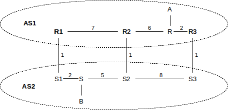
In the absence of the MED, AS1 will send traffic from A to B via the R3–S3 link, and AS2 will return the traffic via S1–R1. These are the links that are closest to R and S, respectively, representing AS1 and AS2’s desire to hand off the outbound traffic as quickly as possible.

However, AS1’s R1, R2 and R3 can provide MED values to AS2 when advertising destination A, indicating a preference for AS2→AS1 traffic to use the rightmost link:

• R1: destination A has MED 200
• R2: destination A has MED 150
• R3: destination A has MED 100

If this is done, and AS2 abides by this information, then AS2 will route traffic from B to A via the S3–R3 link; that is, via the link with the lowest MED value. Note the importance of fact that AS2 is allowed to ignore the MED; use of it may shift costs from AS1 to AS2!

The relative order of the MED values for R1 and R2 is irrelevant, unless the R3–S3 link becomes disabled, in which case the numeric MED values above would mean that AS2 should then prefer the R2–S2 link for reaching A.

There is no way to use MED values to cause A–B traffic to take the R2–S2 link; that link is the minimal-cost link only in the global sense, and the only way to achieve global cost minimization is for the two AS’s to agree to use a common distance metric and a common metric-based routing algorithm, in effect becoming one AS. While AS1 does provide different numeric MED values for the three cross-links, they are used only in ranking precedence, not as numeric measures of cost (though they are sometimes derived from that).

As a hypothetical example of why a site might use the MED, suppose site B in the diagram above wants its customers to experience high-performance downloads. It contracts with AS2, which advertises superior quality in the downloads experienced by users connecting to servers in its domain. In order to achieve this superior quality, it builds a particularly robust network S1–S–S2–S3. It then agrees to accept MED information from other providers so that it can keep outbound traffic in its own network as long as possible, instead of handing it off to other networks of lower quality. AS2 would thus want B→A traffic to travel via S3 to maximize the portion of the path under its own control.

In the example above, the MED values are used to decide between multiple routes to the same destination that all pass through the same AS, namely AS1. Some BGP implementations allow the use of MED values to decide between different routes through different neighbor AS’s. The different neighbors must all have the same local_preference values. For example, AS2 might connect to AS3 and AS4 and receive the following BGP information:

• AS3: destination A has MED 200
• AS4: destination A has MED 100

Assuming AS2 assigns the same local_preference to AS3 and AS4, it might be configured to use these MED values as the tie-breaker, and thus routing traffic to A via AS3.

On Cisco routers, the always-compare-med command is used to create this behavior.

MED values are not intended to be used to communicate routing preferences to non-neighboring AS’s.

Additional information on the use of MED values can be found in RFC 4451.

10.6.5.4   COMMUNITY

This is simply a tag to attach to routes. Routes can have multiple tags corresponding to membership in multiple communities. Some communities are defined globally; for example, NO_EXPORT and NO_ADVERTISE. A route marked with one of these two communities will not be shared further. Other communities may be relevant only to a particular AS.

The importance of communities is that they allow one AS to place some of its routes into specific categories when advertising them to another AS; the categories must have been created and recognized by the receiving AS. The receiving AS is not obligated to honor the community memberships, of course, but doing so has the effect of allowing the original AS to “configure itself” without involving the receiving AS in the process. Communities are often used, for example, by (large) customers of an ISP to request specific routing treatment.

A customer would have to find out from the provider what communities the provider defines, and what their numeric codes are. At that point the customer can place itself into the provider’s community at will.

Here are some of the community values once supported by a no-longer-extant ISP that we shall call AS1. The full community value would have included AS1’s AS-number.

value	action
90	set local_preference used by AS1 to 90
100	set local_preference used by AS1 to 100, the default
105	set local_preference used by AS1 to 105
110	set local_preference used by AS1 to 110
990	the route will not leave AS1’s domain; equivalent to NO_EXPORT
991	route will only be exported to AS1’s other customers

10.6.6   BGP Policy and Transit Traffic

Perhaps the most common source of simple policy decisions is whether a site wants to accept transit traffic.

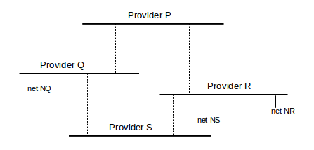
As a first example, let us consider the case of configuring a private link, such as the dashed link1 below between “friendly” but unaffiliated sites A and B:

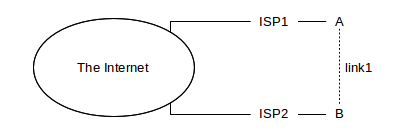
If A and B fully advertise link1, by exporting to their respective ISPs routes to each other, then ISP1 (paid by A) may end up carrying much of B’s traffic or ISP2 (paid by B) may end up carrying much of A’s traffic. Economically, these options are not desirable unless fully agreed to by both parties. The primary issue here is the use of the ISP1–A link by B, and the ISP2–B link by A; use of the shared link1 might be a secondary issue depending on the relative bandwidths and A and B’s understandings of appropriate uses for link1.

Three common options A and B might agree to regarding link1 are no-transit, backup, and load-balancing.

For the no-transit option, A and B simply do not export the route to their respective ISPs at all. This is done via export filtering. If ISP1 does not know A can reach B, it will not send any of B’s traffic to A.

For the backup option, the intent is that traffic to A will normally arrive via ISP1, but if the ISP1 link is down then A’s traffic will be allowed to travel through ISP2 and B. To achieve this, A and B can export their link1-route to each other, but arrange for ISP1 and ISP2 respectively to assign this route a low local_preference value. As long as ISP1 hears of a route to B from its upstream provider, it will reach B that way, and will not advertise the existence of the link1 route to B; ditto ISP2. However, if the ISP2 route to B fails, then A’s upstream provider will stop advertising any route to B, and so ISP1 will begin to use the link1 route to B and begin advertising it to the Internet. The link1 route will be the primary route to B until ISP2’s service is restored.

A and B must convince their respective ISPs to assign the link1 route a low local_preference; they cannot mandate this directly. However, if their ISPs recognize community attributes that, as above, allow customers to influence their local_preference value, then A and B can use this to create the desired local_preference.

For outbound traffic, A and B will need a way to send through one another if their own ISP link is down. One approach is to consider their default-route path (eg to 0.0.0.0/0) to be a concrete destination within BGP. ISP1 advertises this to A, using A’s interior routing protocol, but so does B, and A has configured things so B’s route has a higher cost. Then A will route to 0.0.0.0/0 through ISP1 – that is, will use ISP1 as its default route – as long as it is available, and will switch to B when it is not.

For inbound load balancing, there is no easy fix, in that if ISP1 and ISP2 both export routes to A, then A has lost all control over how other sites will prefer one to the other. A may be able to make one path artificially appear more expensive, and keep tweaking this cost until the inbound loads are comparable. Outbound load-balancing is up to A and B.

Another basic policy question is which of the two available paths site (or regional AS) A uses to reach site D, in the following diagram. B and C are Autonomous Systems.

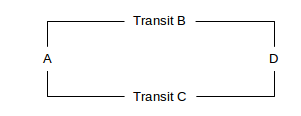
How can A express preference for B over C, assuming B and C both advertise to A their routes to D? Generally A will use a local_preference setting to make the carrier decision for A⟶D traffic, though it is D that makes the decision for the D⟶A traffic. It is possible (though not customary) for one of the transit providers to advertise to A that it can reach D, but not advertise to D that it can reach A.

Here is a similar diagram, showing two transit-providing Autonomous Systems B and C connecting at Internet exchange points IXP1 and IXP2.

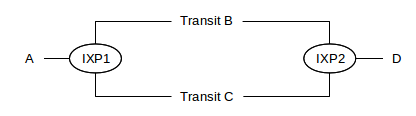
B and C each have routers within each IXP. B would probably like to make sure C does not attempt to save on its long-haul transit costs by forwarding A⟶D traffic over to B at IXP1, and D⟶A traffic over to B at IXP2. B can avoid this problem by not advertising to C that it can reach A and D. In general, transit providers are often quite careful about advertising reachability to any other AS for whom they do not intend to provide transit service, because to do so may implicitly mean getting stuck with that traffic.

If B and C were both to try try to get away with this, a routing loop would be created within IXP1! But in that case in B’s next advertisement to C at IXP1, B would state that it reaches D via AS-path ⟨C⟩ (or ⟨C,D⟩ if D were a full-fledged AS), and C would do similarly; the loop would not continue for long.

10.6.7   BGP Relationships

Arbitrarily complex policies may be created through BGP, and, as we shall see in the following section, convergence to a stable set of routes is not guaranteed. However, most AS policies are determined by a few simple AS business relationships, as identified in [LG01].

Customer-Provider: A provider contracts to transit traffic from the customer to the rest of the Internet. A customer may have multiple providers, for backup or for more efficient routing, but a customer does not accept transit traffic between the providers.

Siblings: Siblings are ISPs that have a connection between them that they intend as a backup route or for internal traffic. Two siblings may or may not have the same upstream ISP provider as parent. The siblings do not use their connection for transit traffic except when one of their primary links is down.

Peers: Peers are two providers that agree to exchange all their customer traffic with each other; thus, peers do use their connection for transit traffic. Generally the idea is for the interconnection to be seen as equally valuable by both parties (eg because the parties exchange comparable volumes of traffic); in such a case there would likely be no exchange of cash, but if the volume flow is significantly asymmetric then compensation can certainly be negotiated.

These business relationships can be described in terms of – or even inferred from – what routes are accepted [LG01]. Every AS has, first of all, its customer routes, that is, the routes of its direct customers, and its customers’ customers, etc. These might be referred to as the ISP’s own routes. Other routes are learned from peers or, sometimes, providers. Essentially every AS exports its customer routes to all its AS neighbors; the issue is with provider routes and peer routes. Here are the rules of [LG01]:

• Customers do not export to their providers routes they have learned from peers or other providers. This would make them into transit providers, which is not their job.
• Providers do export provider/peer routes to their customers (though a provider may just provide a single consolidated default route to a single-homed customer).
• Peers do not export peer or provider routes to other peers; that is, if ISP P1 has peers P2 and P3, and P1 learns of a route to destination D through P2, then P1 does not export that route to P3. Instead, P3 would be expected to have its own relationship with P2, or be a customer of a provider that had a relationship with P2. Peers do not (usually) provide transit services to third parties.
• Siblings do export provider/peer routes to each other, though likely with an understanding about preference values. If S1 and S2 are two siblings with a mutual-backup relationship, and S1 loses its normal connectivity and must rely on the S1–S2 link, then S2 must know all about S1’s routes.
• All AS’s do export their own routes, and their customers’ routes, to customers, siblings, peers and providers.

There may be more complicated variations: if a regional provider is a customer of a large transit backbone, then the backbone might only announce routes listed in transit agreement (rather than all routes, as above). There is a supposition here that the regional provider has multiple connections, and has contracted with that particular transit backbone only for certain routes.

Following these rules creates a simplified BGP world. Special cases for special situations have the potential to introduce non-convergence or instability.

The so-called tier-1 providers are those that are not customers of anyone; these represent the top-level “backbone” providers. Each tier-1 AS must, as a rule, peer with every other tier-1 AS.

A consequence of the use of the above classification and attendant export rules is the no-valley theorem [LG01]: if every AS has BGP policies consistent with the scheme above, then when we consider the full AS-path from A to B, there is at most one peer-peer link. Those to the left of the peer-peer link are (moving from left to right) either customer⟶provider links or sibling⟶sibling links; that is, they are non-downwards (ie upwards or level). To the right of the peer-peer link, we see provider⟶customer or sibling⟶sibling links; that is, these are non-upwards. If there is no peer-peer link, then we can still divide the AS-path into a non-downwards first part and a non-upwards second part.

The above constraints are not quite sufficient to guarantee convergence of the BGP system to a stable set of routes. To ensure convergence in the case without sibling relationships, it is shown in [GR01] that the following simple local_preference rule suffices:

If AS1 gets two routes r1 and r2 to a destination D, and the first AS of the r1 route is a customer of AS1, and the first AS of r2 is not, then r1 will be assigned a higher local_preference value than r2.

More complex rules exist that allow for cases when the local_preference values can be equal; one such rule states that strict inequality is only required when r2 is a provider route. Other straightforward rules handle the case of sibling relationships, eg by requiring that siblings have local_preference rules consistent with the use of their shared connection only for backup.

As a practical matter, unstable BGP arrangements appear rare on the Internet; most actual relationships and configurations are consistent with the rules above.

10.6.8   Examples of BGP Instability

What if the “normal” rules regarding BGP preferences are not followed? It turns out that BGP allows genuinely unstable situations to occur; this is a consequence of allowing each AS a completely independent hand in selecting preference functions. Here are two simple examples, from [GR01].

Example 1: A stable state exists, but convergence to it is not guaranteed. Consider the following network arrangement:

We assume AS1 prefers AS-paths to destination D in the following order:

⟨AS2,AS0⟩, ⟨AS0⟩

That is, ⟨AS2,AS0⟩ is preferred to the direct path ⟨AS0⟩ (one way to express this preference might be “prefer routes for which the AS-PATH begins with AS2”; perhaps the AS1–AS0 link is more expensive). Similarly, we assume AS2 prefers paths to D in the order ⟨AS1,AS0⟩, ⟨AS0⟩. Both AS1 and AS2 start out using path ⟨AS0⟩; they advertise this to each other. As each receives the other’s advertisement, they apply their preference order and therefore each switches to routing D’s traffic to the other; that is, AS1 switches to the route with AS-path ⟨AS2,AS0⟩ and AS2 switches to ⟨AS1,AS0⟩. This, of course, causes a routing loop! However, as soon as they export these paths to one another, they will detect the loop in the AS-path and reject the new route, and so both will switch back to ⟨AS0⟩ as soon as they announce to each other the change in what they use.

This oscillation may continue indefinitely, as long as both AS1 and AS2 switch away from ⟨AS0⟩ at the same moment. If, however, AS1 switches to ⟨AS2,AS0⟩ while AS2 continues to use ⟨AS0⟩, then AS2 is “stuck” and the situation is stable. In practice, therefore, eventual convergence to a stable state is likely.

AS1 and AS2 might choose not to export their D-route to each other to avoid this instability.

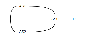
Example 2: No stable state exists. This example is from [VGE00]. Assume that the destination D is attached to AS0, and that AS0 in turn connects to AS1, AS2 and AS3 as in the following diagram:

AS1-AS3 each have a direct route to AS0, but we assume each prefers the AS-path that takes their clockwise neighbor; that is, AS1 prefers ⟨AS3,AS0⟩ to ⟨AS0⟩; AS3 prefers ⟨AS2,AS0⟩ to ⟨AS0⟩, and AS2 prefers ⟨AS1,AS0⟩ to ⟨AS0⟩. This is a peculiar, but legal, example of input filtering.

Suppose all adopt ⟨AS0⟩, and advertise this, and AS1 is the first to look at the incoming advertisements. AS1 switches to the route ⟨AS3,AS0⟩, and announces this.

At this point, AS2 sees that AS1 uses ⟨AS3,AS0⟩; if AS2 switches to AS1 then its path would be ⟨AS1,AS3,AS0⟩ rather than ⟨AS1,AS0⟩ and so it does not make the switch.

But AS3 does switch: it prefers ⟨AS2,AS0⟩ and this is still available. Once it makes this switch, and advertises it, AS1 sees that the route it had been using, ⟨AS3,AS0⟩, has become ⟨AS3,AS1,AS0⟩. At this point AS1 switches back to ⟨AS0⟩.

Now AS2 can switch to using ⟨AS1,AS0⟩, and does so. After that, AS3 finds it is now using ⟨AS2,AS1,AS0⟩ and it switches back to ⟨AS0⟩. This allows AS1 to switch to the longer route, and then AS2 switches back to the direct route, and then AS3 gets the longer route, then AS2 again, etc, forever rotating clockwise.

10.7   Epilog

CIDR was a deceptively simple idea. At first glance it is a straightforward extension of the subnet concept, moving the net/host division point to the left as well as to the right. But it has ushered in true hierarchical routing, most often provider-based. While CIDR was originally offered as a solution to some early crises in IPv4 address-space allocation, it has been adopted into the core of IPv6 routing as well.

Interior routing – using either distance-vector or link-state protocols – is neat and mathematical. Exterior routing with BGP is messy and arbitrary. Perhaps the most surprising thing about BGP is that the Internet works as well as it does, given the complexity of provider interconnections. The business side of routing almost never has an impact on ordinary users. To an extent, BGP works well because providers voluntarily limit the complexity of their filtering preferences, but that seems to be largely because the business relationships of real-world ISPs do not seem to require complex filtering.

10.8   Exercises

1. Consider the following IP forwarding table that uses CIDR. IP address bytes are in hexadecimal, so each hex digit corresponds to four address bits.

destination	next_hop
81.30.0.0/12	A
81.3c.0.0/16	B
81.3c.50.0/20	C
81.40.0.0/12	D
81.44.0.0/14	E

For each of the following IP addresses, indicate to what destination it is forwarded.

(i) 81.3b.15.49

(ii) 81.3c.56.14

(iii) 81.3c.85.2e

(iv) 81.4a.35.29

(v) 81.47.21.97

(vi) 81.43.01.c0

2. Consider the following IP forwarding table, using CIDR. As in exercise 1, IP address bytes are in hexadecimal.

destination	next_hop
00.0.0.0/2	A
40.0.0.0/2	B
80.0.0.0/2	C
C0.0.0.0/2	D

(a). To what next_hop would each of the following be routed? 63.b1.82.15, 9e.00.15.01, de.ad.be.ef

(b). Explain why every IP address is routed somewhere, even though there is no default entry.

3. Give an IPv4 forwarding table – using CIDR – that will route all Class A addresses to next_hop A, all Class B addresses to next_hop B, and all Class C addresses to next_hop C.

4. Suppose a router using CIDR has the following entries. Address bytes are in decimal except for the third byte, which is in binary.

destination	next_hop
37.119.0000 0000.0/18	A
37.119.0100 0000.0/18	A
37.119.1000 0000.0/18	A
37.119.1100 0000.0/18	B

These four entries cannot be consolidated into a single /16 entry, because they don’t all go to the same next_hop. How could they be consolidated into two entries?

5. Suppose P, Q and R are ISPs with respective CIDR address blocks (with bytes in decimal) 51.0.0.0/8, 52.0.0.0/8 and 53.0.0.0/8. P then has customers A and B, to which it assigns address blocks as follows:

A: 51.10.0.0/16

B: 51.23.0.0/16

Q has customers C and D and assigns them address blocks as follows:

C: 52.14.0.0/16

D: 52.15.0.0/16

(a). Give forwarding tables for P, Q and R assuming they connect to each other and to each of their own customers.

(b). Now suppose A switches from provider P to provider Q, and takes its address block with it. Give the forwarding tables for P, Q and R; the longest-match rule will be needed to resolve conflicts.

(c). Now suppose in addition to A switching from P to Q, C switches from provider Q to provider R. Give the forwarding tables.

6. Suppose P, Q and R are ISPs as in the previous problem. P and R do not connect directly; they route traffic to one another via Q. In addition, customer B is multi-homed and has a secondary connection to provider R; customer D is also multi-homed and has a secondary connection to provider P; these secondary connections are not advertised to other providers however. Give forwarding tables for P, Q and R.

7. Consider the following network of providers P-S, all using BGP. The providers are the horizontal lines; each provider is its own AS.

(a). What routes to network NS will P receive, assuming there is no export filtering? For each route, list the AS-path.

(b). What routes to network NQ will P receive? For each route, list the AS-path.

(c). Suppose R uses export filtering so as not to advertise to P any of its routes except those that involve S in their AS-path. What routes to network NR will P receive, with AS-paths?

8. Consider the following network of Autonomous Systems AS1 through AS6, which double as destinations. When AS1 advertises itself to AS2, for example, the AS-path it provides is ⟨AS1⟩.

AS1────────AS2────────AS3
 │                     :
 │                     :
 │                     :
AS4────────AS5────────AS6

(a). If neither AS3 nor AS6 exports their AS3–AS6 link to their neighbors AS2 and AS5 to the left, what routes will AS2 receive to reach AS5? Specify routes by AS-path.

(b). What routes will AS2 receive to reach AS6?

(c). Suppose AS3 exports to AS2 its link to AS6, but AS6 continues not to export the AS3–AS6 link to AS5. How will AS5 now reach AS2? How will AS2 now reach AS6? Assume that there are no local preferences in use in BGP best-path selection, and that the shortest AS-path wins.

9. Suppose that Internet routing in the US used geographical routing, and the first 12 bits of every IP address represent a geographical area similar in size to a telephone area code. Megacorp gets the prefix 12.34.0.0/16, based geographically in Chicago, and allocates subnets from this prefix to its offices in all 50 states. Megacorp routes all its internal traffic over its own network.

(a). Assuming all Megacorp traffic must enter and exit in Chicago, what is the route of traffic to and from the San Diego office to a client also in San Diego?

(b). Now suppose each office has its own link to a local ISP, but still uses its 12.34.0.0/16 IP addresses. Now what is the route of traffic between the San Diego office and its neighbor?

(c). Suppose Megacorp gives up and gets a separate geographical prefix for each office. What must it do to ensure that its internal traffic is still routed over its own network?

10. Suppose we try to use BGP’s strategy of exchanging destinations plus paths as an interior routing-update strategy, perhaps replacing distance-vector routing. No costs or hop-counts are used, but routers attach to each destination a list of the routers used to reach that destination. Routers can also have route preferences, such as “prefer my link to B whenever possible”.

(a). Consider the network of 9.2   Distance-Vector Slow-Convergence Problem:

D───────────A───────────B

The D–A link breaks, and B offers A what it thinks is its own route to D. Explain how exchanging path information prevents a routing loop here.

(b). Suppose the network is as below, and initially each router knows about itself and its immediately adjacent neighbors. What sequence of router announcements can lead to A reaching F via A→D→E→B→C→F, and what individual router preferences would be necessary? (Initially, for example, A would reach B directly; what preference might make it prefer A→D→E→B?)

A────────B────────C
│        │        │
│        │        │
│        │        │
D────────E────────F

(c). Explain why this method is equivalent to distance-vector with the hopcount metric, if routers are not allowed to have preferences and if the router-path length is used as a tie-breaker.