3 Other LANs
In the wired era, one could get along quite well with nothing but Ethernet and the occasional long-haul point-to-point link joining different sites. However, there are important alternatives out there. Some, like token ring, are mostly of historical importance; others, like virtual circuits, are of great conceptual importance but – so far – of only modest day-to-day significance.
And then there is wireless. It would be difficult to imagine contemporary laptop networking, let alone mobile devices, without it. In both homes and offices, Wi-Fi connectivity is the norm. A return to being tethered by wires is almost unthinkable.
3.1 Virtual Private Network
Suppose you want to connect to your workplace network from home. Your workplace, however, has a security policy that does not allow “outside” IP addresses to access essential internal resources. How do you proceed, without leasing a dedicated telecommunications line to your workplace?
A virtual private network, or VPN, provides a solution; it supports creation of virtual links that join far-flung nodes via the Internet. Your home computer creates an ordinary Internet connection (TCP or UDP) to a workplace VPN server (IP-layer packet encapsulation can also be used; see 7.11 Mobile IP). Each end of the connection is associated with a software-created virtual network interface; each of the two virtual interfaces is assigned an IP address. When a packet is to be sent along the virtual link, it is actually encapsulated and sent along the original Internet connection to the VPN server, wending its way through the commodity Internet; this process is called tunneling. To all intents and purposes, the virtual link behaves like any other physical link.
Tunneled packets are usually encrypted as well as encapsulated, though that is a separate issue. One example of a tunneling protocol is to treat a TCP home-workplace connection as a serial line and send packets over it back-to-back, using PPP with HDLC; see 4.1.5.1 HDLC and RFC 1661.
At the workplace side, the virtual network interface in the VPN server is attached to a router or switch; at the home user’s end, the virtual network interface can now be assigned an internal workplace IP address. The home computer is now, for all intents and purposes, part of the internal workplace network.
In the diagram below, the user’s regular Internet connection is via hardware interface eth0. A connection is established to Site A’s VPN server; a virtual interface tun0 is created on the user’s machine which appears to be a direct link to the VPN server. The tun0 interface is assigned a Site-A IP address. Packets sent via the tun0 interface in fact travel over the original connection via eth0 and the Internet.
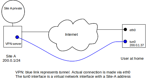
After the VPN is set up, the home host’s tun0 interface appears to be locally connected to Site A, and thus the home host is allowed to connect to the private area within Site A. The home host’s forwarding table will be configured so that traffic to Site A’s private addresses is routed via interface tun0.
VPNs are also commonly used to connect entire remote offices to headquarters. In this case the remote-office end of the tunnel will be at that office’s local router, and the tunnel will carry traffic for all the workstations in the remote office.
To improve security, it is common for the residential (or remote-office) end of the VPN connection to use the VPN connection as the default route for all traffic except that needed to maintain the VPN itself. This may require a so-called host-specific forwarding-table entry at the residential end to allow the packets that carry the VPN tunnel traffic to be routed correctly via eth0. This routing strategy means that potential intruders cannot access the residential host – and thus the workplace internal network – through the original residential Internet access. A consequence is that if the home worker downloads a large file from a non-workplace site, it will travel first to the workplace, then back out to the Internet via the VPN connection, and finally arrive at the home.
3.2 Carrier Ethernet
Carrier Ethernet is a leased-line point-to-point link between two sites, where the subscriber interface at each end of the line looks like Ethernet (in some flavor). The physical path in between sites, however, need not have anything to do with Ethernet; it may be implemented however the carrier wishes. In particular, it will be (or at least appear to be) full-duplex, it will be collision-free, and its length may far exceed the maximum permitted by any IEEE Ethernet standard.
Bandwidth can be purchased in whatever increments the carrier has implemented. The point of carrier Ethernet is to provide a layer of abstraction between the customers, who need only install a commodity Ethernet interface, and the provider, who can upgrade the link implementation at will without requiring change at the customer end.
In a sense, carrier Ethernet is similar to the widespread practice of provisioning residential DSL and cable routers with an Ethernet interface for customer interconnection; again, the actual link technologies may not look anything like Ethernet, but the interface will.
A carrier Ethernet connection looks like a virtual VPN link, but runs on top of the provider’s internal network rather than the Internet at large. Carrier Ethernet connections often provide the primary Internet connectivity for one endpoint, unlike Internet VPNs which assume both endpoints already have full Internet connectivity.
3.3 Wi-Fi
Wi-Fi is a trademark denoting any of several IEEE wireless-networking protocols in the 802.11 family, specifically 802.11a, 802.11b, 802.11g, 802.11n, and 802.11ac. Like classic Ethernet, Wi-Fi must deal with collisions; unlike Ethernet, however, Wi-Fi is unable to detect collisions in progress, complicating the backoff and retransmission algorithms. Wi-Fi is designed to interoperate freely with Ethernet at the logical LAN layer; that is, Ethernet and Wi-Fi traffic can be freely switched from the wired side to the wireless side.
Generally, Wi-Fi uses the 2.4 GHz ISM (Industrial, Scientific and Medical) band used also by microwave ovens, though 802.11a uses a 5 GHz band, 802.11n supports that as an option and the new 802.11ac has returned to using 5 GHz exclusively. The 5 GHz band has reduced ability to penetrate walls, often resulting in a lower effective range. Wi-Fi radio spectrum is usually unlicensed, meaning that no special permission is needed to transmit but also that others may be trying to use the same frequency band simultaneously; the availability of unlicensed channels in the 5 GHz band continues to evolve.
The table below summarizes the different Wi-Fi versions. All bit rates assume a single spatial stream; channel widths are nominal.
| IEEE name | maximum bit rate | frequency | channel width |
|---|---|---|---|
| 802.11a | 54 Mbps | 5 GHz | 20 MHz |
| 802.11b | 11 Mbps | 2.4 GHz | 20 MHz |
| 802.11g | 54 Mbps | 2.4 GHz | 20 MHz |
| 802.11n | 65-150 Mbps | 2.4/5 GHz | 20-40 MHz |
| 802.11ac | 78-867 Mbps | 5 GHz | 20-160 MHz |
The maximum bit rate is seldom achieved in practice. The effective bit rate must take into account, at a minimum, the time spent in the collision-handling mechanism. More significantly, all the Wi-Fi variants above use dynamic rate scaling, below; the bit rate is reduced up to tenfold (or more) in environments with higher error rates, which can be due to distance, obstructions, competing transmissions or radio noise. All this means that, as a practical matter, getting 150 Mbps out of 802.11n requires optimum circumstances; in particular, no competing senders and unimpeded line-of-sight transmission. 802.11n lower-end performance can be as little as 10 Mbps, though 40-100 Mbps (for a 40 MHz channel) may be more typical.
The 2.4 GHz ISM band is divided by international agreement into up to 14 officially designated channels, each about 5 MHz wide, though in the United States use may be limited to the first 11 channels. The 5 GHz band is similarly divided into 5 MHz channels. One Wi-Fi sender, however, needs several of these official channels; the typical 2.4 GHz 802.11g transmitter uses an actual frequency range of up to 22 MHz, or up to five channels. As a result, to avoid signal overlap Wi-Fi use in the 2.4 GHz band is often restricted to official channels 1, 6 and 11. The end result is that unrelated Wi-Fi transmitters can and do interact with and interfere with each other.
The United States requires users of the 5 GHz band to avoid interfering with weather and military applications in the same frequency range. Once that is implemented, however, there are more 5 MHz channels at this frequency than in the 2.4 GHz ISM band, which is one of the reasons 802.11ac can run faster (below).
Wi-Fi designers can improve speed through a variety of techniques, including
- improved radio modulation techniques
- improved error-correcting codes
- smaller guard intervals between symbols
- increasing the channel width
- allowing multiple spatial streams via multiple antennas
The first two in this list seem by now to be largely tapped out; the third reduces the range but may increase the data rate by 11%.
The largest speed increases are obtained by increasing the number of 5 MHz channels used. For example, the 65 Mbps bit rate above for 802.11n is for a nominal frequency range of 20 MHz, comparable to that of 802.11g. However, in areas with minimal competition from other signals, 802.11n supports using a 40 MHz frequency band; the bit rate then goes up to 135 Mbps (150 Mbps with a smaller guard interval). This amounts to using two of the three available 2.4 GHz Wi-Fi bands. Similarly, the wide range in 802.11ac bit rates reflects support for using channel widths ranging from 20 MHz up to 160 MHz (32 5-MHz official channels).
For all the categories in the table above, additional bits are used for error-correcting codes. For 802.11g operating at 54 Mbps, for example, the actual raw bit rate is (4/3)×54 = 72 Mbps, sent in symbols consisting of six bits as a unit.
3.3.1 Multiple Spatial Streams
The latest innovation in improving Wi-Fi data rates is to support multiple spatial streams, through an antenna technique known as multiple-input-multiple output, or MIMO. To use N streams, both sender and receiver must have N antennas; all the antennas use the same frequency channels but each transmitter antenna sends a different data stream. While the antennas are each more-or-less omnidirectional, careful signal analysis at the receiver can in principle recover each data stream. In practice, overall data-rate improvement over a single antenna can be considerably less than N.
The 802.11n standard allows for up to four spatial streams, for a theoretical maximum bit rate of 600 Mbps. 802.11ac allows for up to eight spatial streams, for an even-more-theoretical maximum of close to 7 Gbps. MIMO support is sometimes described with an A×B×C notation, eg 3×3×2, where A and B are the number of transmitting and receiving antennas and C ≤ min(A,B) is the number of spatial streams.
3.3.2 Wi-Fi and Collisions
We looked extensively at the 10 Mbps Ethernet collision-handling mechanisms in 2.1 10-Mbps classic Ethernet, only to conclude that with switches and full-duplex links, Ethernet collisions are rapidly becoming a thing of the past. Wi-Fi, however, has brought collisions back from obscurity. While there is a largely-collision-free mode for Wi-Fi operation (3.3.7 Wi-Fi Polling Mode), it is not commonly used, and collision management has a significant impact on ordinary Wi-Fi performance.
Wi-Fi, like almost any other wireless protocol, cannot detect collisions in progress. This has to do with the relative signal strength of the remote signal at the local transmitter. Along a wire-based Ethernet the remote signal might be as weak as 1/100 of the transmitted signal but that 1% received signal is still detectable during transmission. However, with radio the remote signal might easily be as little as 1/100,000 of the transmitted signal, and it is simply overwhelmed during transmission. Thus, while the Ethernet algorithm was known as CSMA/CD, where CD stood for Collision Detection, Wi-Fi uses CSMA/CA, where CA stands for Collision Avoidance.
The basic collision-avoidance algorithm is as follows. There are three parameters applicable here (values are for 802.11b/g in the 2.4 GHz band); the value we call IFS is more formally known as DIFS (D for “distributed”; see 3.3.7 Wi-Fi Polling Mode).
- slot time: 20 µsec
- IFS, the “normal” InterFrame Spacing: 50 µsec
- SIFS, the short IFS: 10 µsec
A sender wanting to send a new data packet waits the IFS time after first sensing the medium to see if it is idle. If no other traffic is seen in this interval, the station may then transmit immediately. However, if other traffic is sensed, the sender waits for the other traffic to finish and then for one IFS time after. If the station had to wait for other traffic, even briefly, it must then do an exponential backoff even for its first transmission attempt; other stations, after all, are likely also waiting, and avoiding an initial collision is strongly preferred.
The initial backoff is to choose a random k<25 = 32 (recall that classic Ethernet in effect chooses an initial backoff of k<20 = 1; ie k=0). The prospective sender then waits k slot times. While waiting, the sender continues to monitor for other traffic; if any other transmission is detected, then the sender “suspends” the backoff-wait clock. The clock resumes when the other transmission has completed and one followup idle interval of length IFS has elapsed. Under this rule, the backoff-wait clock can expire only when the clock is running and therefore the medium is idle, at which point the transmission begins.
If there is a collision, the station retries, after doubling the backoff range to 64, then 128, 256, 512, 1024 and again 1024. If these seven attempts all fail, the packet is discarded and the sender starts over.
In one slot time, radio signals move 6,000 meters; the Wi-Fi slot time – unlike that for Ethernet – has nothing to do with the physical diameter of the network. As with Ethernet, though, the Wi-Fi slot time represents the fundamental unit for backoff intervals.
Finally, we note that, unlike Ethernet collisions, Wi-Fi collisions are a local phenomenon: if A and B transmit simultaneously, a collision occurs at node C only if the signals of A and B are both strong enough at C to interfere with one another. It is possible that a collision occurs at station C midway between A and B, but not at station D that is close to A. We return to this in 3.3.2.2 Hidden-Node Problem.
Because Wi-Fi cannot detect collisions directly, the protocol adds link-layer ACK packets (unrelated to the later TCP ACK), at least for unicast transmission. Once a station has received a packet addressed to it, it waits for time SIFS and sends the ACK; at the instant when the end of the SIFS interval is reached, the receiver will be the only station authorized to send. Any other stations waiting the longer IFS period will see the ACK before the IFS time has elapsed and will thus not interfere with the ACK; similarly, any stations with a running backoff-wait clock will continue to have that clock suspended.
3.3.2.1 Wi-Fi RTS/CTS
Wi-Fi stations optionally also use a request-to-send/clear-to-send (RTS/CTS) protocol. Usually this is used only for larger packets; often, the RTS/CTS “threshold” (the size of the largest packet not sent using RTS/CTS) is set (as part of the Access Point configuration) to be the maximum packet size, effectively disabling this feature. The idea here is that a large packet that is involved in a collision represents a significant waste of potential throughput; for large packets, we should ask first.
The RTS packet – which is small – is sent through the normal procedure outlined above; this packet includes the identity of the destination and the size of the data packet the station desires to transmit. The destination station then replies with CTS after the SIFS wait period, effectively preventing any other transmission after the RTS. The CTS packet also contains the data-packet size. The original sender then waits for SIFS after receiving the CTS, and sends the packet. If all other stations can hear both the RTS and CTS messages, then once the RTS and CTS are sent successfully no collisions should occur during packet transmission, again because the only idle times are of length SIFS and other stations should be waiting for time IFS.
3.3.2.3 Wi-Fi Fragmentation
Conceptually related to RTS/CTS is Wi-Fi fragmentation. If error rates or collision rates are high, a sender can send a large packet as multiple fragments, each receiving its own link-layer ACK. As we shall see in 5.3.1 Error Rates and Packet Size, if bit-error rates are high then sending several smaller packets often leads to fewer total transmitted bytes than sending the same data as one large packet.
Wi-Fi packet fragments are reassembled by the receiving node, which may or may not be the final destination.
As with the RTS/CTS threshold, the fragmentation threshold is often set to the size of the maximum packet. Adjusting the values of these thresholds is seldom necessary, though might be appropriate if monitoring revealed high collision or error rates. Unfortunately, it is essentially impossible for an individual station to distinguish between reception errors caused by collisions and reception errors caused by other forms of noise, and so it is hard to use reception statistics to distinguish between a need for RTS/CTS and a need for fragmentation.
3.3.3 Dynamic Rate Scaling
Wi-Fi senders, if they detect transmission problems, are able to reduce their transmission bit rate in a process known as rate scaling or rate control. The idea is that lower bit rates will have fewer noise-related errors, and so as the error rate becomes unacceptably high – perhaps due to increased distance – the sender should fall back to a lower bit rate. For 802.11g, the standard rates are 54, 48, 36, 24, 18, 12, 9 and 6 Mbps. Senders attempt to find the transmission rate that maximizes throughput; for example, 36 Mbps with a packet loss rate of 25% has an effective throughput of 36 × 75% = 27 Mbps, and so is better than 24 Mbps with no losses.
Senders may update their bit rate on a per-packet basis; senders may also choose different bit rates for different recipients. For example, if a sender sends a packet and receives no confirming link-layer ACK (described below), the sender may fall back to the next lower bit rate. The actual bit-rate-selection algorithm lives in the particular Wi-Fi driver in use; different nodes in a network may use different algorithms. A variety of algorithms have been proposed; a typical strategy involves maintaining a running average of the transmission success rate for each bit-rate in recent use. See [JB05] for a summary. While the signal-to-noise ratio has a strong influence on the transmission success rate, the exact correlation is sometimes obscure, and drivers do not use the signal-to-noise ratio directly.
While lowering the bit rate likely does increase transmission reliability in the face of noise, the longer packet-transmission times caused by the lower bit rate may increase the frequency of hidden-node collisions.
Because the actual data in a Wi-Fi packet may be sent at a rate not every participant is close enough to receive correctly, every Wi-Fi transmission begins with a brief preamble at the minimum bit rate.
3.3.4 Wi-Fi Configurations
There are two common Wi-Fi configurations: infrastructure and ad hoc. The latter includes individual Wi-Fi-equipped nodes communicating informally; for example, two laptops can set up an ad hoc connection to transfer data at a meeting. Ad hoc connections are often used for very simple networks not providing Internet connectivity. Complex ad hoc networks are, however, certainly possible; see 3.3.8 MANETs.
The more-common infrastructure configuration involves designated access points to which individual Wi-Fi stations must associate before general communication can begin. The association process – carried out by an exchange of special management packets – may be restricted to stations with hardware (“MAC”) addresses on a predetermined list, or to stations with valid cryptographic credentials. Stations may regularly re-associate to their Access Point, especially if they wish to communicate some status update.
Stations in an infrastructure network communicate directly only with their access point. If B and C share access point A, and B wishes to send a packet to C, then B first forwards the packet to A and A then forwards it to C. While this introduces a degree of inefficiency, it does mean that the access point and its associated nodes automatically act as a true LAN: every node can reach every other node. In an ad hoc network, by comparison, it is quite common for two nodes to be able to reach each other only by forwarding through an intermediate third node; this is in fact exactly the hidden-node scenario.
Finally, Wi-Fi is by design completely interoperable with Ethernet; if station A is associated with access point AP, and AP also connects via (cabled) Ethernet to station B, then if A wants to send a packet to B it sends it using AP as the Wi-Fi destination but with B also included in the header as the “actual” destination. Once it receives the packet by wireless, AP acts as an Ethernet switch and forwards the packet to B.
3.3.5 Wi-Fi Roaming
Wi-Fi access points are generally identified by their SSID, an administratively defined string such as “linksys” or “loyola”. These are periodically broadcast by the access point in special beacon packets (though for pseudo-security reasons beacon packets can be suppressed). Large installations can create “roaming” access among multiple access points by assigning all the access points the same SSID. An individual station will stay with the access point with which it originally associated until the signal strength falls below a certain level, at which point it will seek out other access points with the same SSID and with a stronger signal. In this way, a large area can be carpeted with multiple Wi-Fi access points, so as to look like one large Wi-Fi domain.
In order for this to work, traffic to wireless node B must find B’s current access point AP. This is done in much the same way as, in a wired Ethernet, traffic finds a laptop that has been unplugged, carried to a new building, and plugged in again. The distribution network is the underlying wired network (eg Ethernet) to which all the access points connect. If the distribution network is a switched Ethernet supporting the usual learning mechanism (2.4 Ethernet Switches), then Wi-Fi location update is straightforward. Suppose B is a wireless node that has been exchanging packets via the distribution network with C (perhaps a router connecting B to the Internet). When B moves to a new access point, all it has to do is send any packet over the LAN to C, and the Ethernet switches involved will then learn the route through the switched Ethernet from C to B’s current AP, and thus to B.
This process may leave other switches – not currently communicating with B – still holding in their forwarding tables the old location for B. This is not terribly serious, but can be avoided entirely if, after moving, B sends out an Ethernet broadcast packet.
Ad hoc networks also have SSIDs; these are generated pseudorandomly at startup. Ad hoc networks have beacon packets as well; all nodes participate in the regular transmission of these via a distributed algorithm.
3.3.6 Wi-Fi Security
Wi-Fi traffic is visible to anyone nearby with an appropriate receiver; this eavesdropping zone can be expanded by use of a larger antenna. Because of this, Wi-Fi security is important, and Wi-Fi supports several types of traffic encryption.
The original Wired-Equivalent Privacy, or WEP, encryption standard, contained a fatal (and now-classic) flaw. Bytes of the key could be could be “broken” – that is, guessed – sequentially. Knowing bytes 0 through i−1 would allow an attacker to guess byte i with a relatively small amount of data, and so on through the entire key.
WEP has been replaced with Wi-Fi Protected Access, or WPA; the current version is WPA2. WPA2 encryption is believed to be quite secure, although there was a vulnerability in the associated Wi-Fi Protected Setup protocol.
Key management, however, can be a problem. Many smaller sites use “pre-shared key” mode, known as WPA-Personal, in which a single key is entered into the Access Point (ideally not over the air) and into each connecting station. The key is usually a hash of a somewhat longer passphrase. The use of a common key for multiple stations makes changing the key, or revoking the key for a particular user, difficult.
A more secure approach is WPA-Enterprise; this allows each station to have a separate key, and also for each station key to be recognized by all access points. It is part of the IEEE 802.1X security framework (technically so is WPA-Personal, though a much smaller part). In this model, the client node is known as the supplicant, the Access Point is known as the authenticator, and there is a third system involved known as the authentication server. One authentication server can support multiple access points.
To begin the association process, the supplicant contacts the authenticator using the Extensible Authentication Protocol, or EAP, with what amounts to a request to associate to that access point. EAP is a generic message framework meant to support multiple specific types of authentication; see RFC 3748 and RFC 5247. The EAP request is forwarded to an authentication server, which may exchange (via the authenticator) several challenge/response messages with the supplicant. EAP is usually used in conjunction with the RADIUS (Remote Authentication Dial-In User Service) protocol (RFC 2865), which is a specific (but flexible) authentication-server protocol. WPA-Enterprise is sometimes known as 802.1X mode, EAP mode or RADIUS mode.
One peculiarity of EAP is that EAP communication takes place before the supplicant is given an IP address (in fact before the supplicant has completed associating itself to the access point); thus, a mechanism must be provided to support exchange of EAP packets between supplicant and authenticator. This mechanism is known as EAPOL, for EAP Over LAN. EAP messages between the authenticator and the authentication server, on the other hand, can travel via IP; in fact, sites may choose to have the authentication server hosted remotely.
Once the authentication server (eg RADIUS server) is set up, specific per-user authentication methods can be entered. This can amount to ⟨username,password⟩ pairs, or some form of security certificate, or often both. The authentication server will generally allow different encryption protocols to be used for different supplicants, thus allowing for the possibility that there is not a common protocol supported by all stations.
When this authentication strategy is used, the access point no longer needs to know anything about what authentication protocol is actually used; it is simply the middleman forwarding EAP packets between the supplicant and the authentication server. The access point allows the supplicant to associate into the network once it receives permission to do so from the authentication server.
3.3.7 Wi-Fi Polling Mode
Wi-Fi also includes a “polled” mechanism, where one station (the Access Point) determines which stations are allowed to send. While it is not often used, it has the potential to greatly reduce collisions, or even eliminate them entirely. This mechanism is known as “Point Coordination Function”, or PCF, versus the collision-oriented mechanism which is then known as “Distributed Coordination Function”. The PCF name refers to the fact that in this mode it is the Access Point that is in charge of coordinating which stations get to send when.
The PCF option offers the potential for regular traffic to receive improved throughput due to fewer collisions. However, it is often seen as intended for real-time Wi-Fi traffic, such as voice calls over Wi-Fi.
The idea behind PCF is to schedule, at regular intervals, a contention-free period, or CFP. During this period, the Access Point may
- send Data packets to any receiver
- send Poll packets to any receiver, allowing that receiver to reply with its own data packet
- send a combination of the two above (not necessarily to the same receiver)
- send management packets, including a special packet marking the end of the CFP
None of these operations can result in a collision (unless an unrelated but overlapping Wi-Fi domain is involved).
Stations receiving data from the Access Point send the usual ACK after a SIFS interval. A data packet from the Access Point addressed to station B may also carry, piggybacked in the Wi-Fi header, a Poll request to station C; this saves a transmission. Polled stations that send data will receive an ACK from the Access Point; this ACK may be combined in the same packet with the Poll request to the next station.
At the end of the CFP, the regular “contention period” or CP resumes, with the usual CSMA/CA strategy. The time interval between the start times of consecutive CFP periods is typically 100 ms, short enough to allow some real-time traffic to be supported.
During the CFP, all stations normally wait only the Short IFS, SIFS, between transmissions. This works because normally there is only one station designated to respond: the Access Point or the polled station. However, if a station is polled and has nothing to send, the Access Point waits for time interval PIFS (PCF Inter-Frame Spacing), of length midway between SIFS and IFS above (our previous IFS should now really be known as DIFS, for DCF IFS). At the expiration of the PIFS, any non-Access-Point station that happens to be unaware of the CFP will continue to wait the full DIFS, and thus will not transmit. An example of such a CFP-unaware station might be one that is part of an entirely different but overlapping Wi-Fi network.
The Access Point generally maintains a polling list of stations that wish to be polled during the CFP. Stations request inclusion on this list by an indication when they associate or (more likely) reassociate to the Access Point. A polled station with nothing to send simply remains quiet.
PCF mode is not supported by many lower-end Wi-Fi routers, and often goes unused even when it is available. Note that PCF mode is collision-free, so long as no other Wi-Fi access points are active and within range. While the standard has some provisions for attempting to deal with the presence of other Wi-Fi networks, these provisions are somewhat imperfect; at a minimum, they are not always supported by other access points. The end result is that polling is not quite as useful as it might be.
3.3.8 MANETs
The MANET acronym stands for mobile ad hoc network; in practice, the term generally applies to ad hoc wireless networks of sufficient complexity that some internal routing mechanism is needed to enable full connectivity. The term mesh network is also used. While MANETs can use any wireless mechanism, we will assume here that Wi-Fi is used.
MANET nodes communicate by radio signals with a finite range, as in the diagram below.
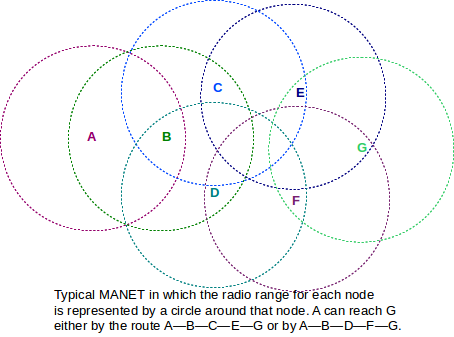
Each node’s radio range is represented by a circle centered about that node. In general, two MANET nodes may be able to communicate only by relaying packets through intermediate nodes, as is the case for nodes A and G in the diagram above.
In the field, the radio range of each node may not be very circular, due to among other things signal reflection and blocking from obstructions. An additional complication arises when the nodes (or even just obstructions) are moving in real time (hence the “mobile” of MANET); this means that a working route may stop working a short time later. For this reason, and others, routing within MANETs is a good deal more complex than routing in an Ethernet. A switched Ethernet, for example, is required to be loop-free, so there is never a choice among multiple alternative routes.
Note that, without successful LAN-layer routing, a MANET does not have full node-to-node connectivity and thus does not meet the definition of a LAN given in 1.9 LANs and Ethernet. With either LAN-layer or IP-layer routing, one or more MANET nodes may serve as gateways to the Internet.
Note also that MANETs in general do not support broadcast, unless the forwarding of broadcast messages throughout the MANET is built in to the routing mechanism. This can complicate the assignment of IP addresses; the common IPv4 mechanism we will describe in 7.8 Dynamic Host Configuration Protocol (DHCP) relies on broadcast and so usually needs some adaptation.
Finally, we observe that while MANETs are of great theoretical interest, their practical impact has been modest; they are almost unknown, for example, in corporate environments. They appear most useful in emergency situations, rural settings, and settings where the conventional infrastructure network has failed or been disabled.
3.3.8.1 Routing in MANETs
Routing in MANETs can be done either at the LAN layer, using physical addresses, or at the IP layer with some minor bending of the rules.
Either way, nodes must find out about the existence of other nodes, and appropriate routes must then be selected. Route selection can use any of the mechanisms we describe later in 9 Routing-Update Algorithms.
Routing at the LAN layer is much like routing by Ethernet switches; each node will construct an appropriate forwarding table. Unlike Ethernet, however, there may be multiple paths to a destination, direct connectivity between any particular pair of nodes may come and go, and negotiation may be required even to determine which MANET nodes will serve as forwarders.
Routing at the IP layer involves the same issues, but at least IP-layer routing-update algorithms have always been able to handle multiple paths. There are some minor issues, however. When we initially presented IP forwarding in 1.10 IP - Internet Protocol, we assumed that routers made their decisions by looking only at the network prefix of the address; if another node had the same network prefix it was assumed to be reachable directly via the LAN. This model usually fails badly in MANETs, where direct reachability has nothing to do with addresses. At least within the MANET, then, a modified forwarding algorithm must be used where every address is looked up in the forwarding table. One simple way to implement this is to have the forwarding tables contain only host-specific entries as were discussed in 3.1 Virtual Private Network.
Multiple routing algorithms have been proposed for MANETs. Performance of a given algorithm may depend on the following factors:
- The size of the network
- Whether some nodes have agreed to serve as routers
- The degree of node mobility, especially of routing-node mobility if applicable
- Whether the nodes are under common administration, and thus may agree to defer their own transmission interests to the common good
- per-node storage and power availability
3.4 WiMAX
WiMAX is a wireless network technology standardized by IEEE 802.16. It supports both stationary subscribers (802.16d) and mobile subscribers (802.16e). The stationary-subscriber version is often used to provide residential Internet connectivity, in both urban and rural areas. The mobile version is sometimes referred to as a “fourth generation” or 4G networking technology; its similar primary competitor is known as LTE. WiMAX is used in many mobile devices, from smartphones to traditional laptops with wireless cards installed.
As in the sidebar at the start of 3.3 Wi-Fi we will use the term “data rate” for what is commonly called “bandwidth” to avoid confusion with the radio-specific meaning of the latter term.
WiMAX can use unlicensed frequencies, like Wi-Fi, but its primary use is over licensed radio spectrum. WiMAX also supports a number of options for the width of its frequency band; the wider the band, the higher the data rate. Wider bands also allow the opportunity for multiple independent frequency channels. Downlink (base station to subscriber) data rates can be well over 100 Mbps (uplink rates are usually smaller).
Like Wi-Fi, WiMAX subscriber stations connect to a central access point, though the WiMAX standard prefers the term base station which we will use henceforth. Stationary-subscriber WiMAX, however, operates on a much larger scale. The coverage radius of a WiMAX base station can be tens of kilometers if larger antennas are provided, versus less (sometimes much less) than 100 meters for Wi-Fi; mobile-subscriber WiMAX might have a radius of one or two kilometers. Large-radius base stations are typically mounted in towers. Subscriber stations are not generally expected to be able to hear other stations; they interact only with the base station. As WiMAX distances increase, the data rate is reduced.
As with Wi-Fi, the central “contention” problem is how to schedule transmissions of subscriber stations so they do not overlap; that is, collide. The base station has no difficulty broadcasting transmissions to multiple different stations sequentially; it is the transmissions of those stations that must be coordinated. Once a station completes the network entry process to connect to a base station (below), it is assigned regular (though not necessarily periodic) transmission slots. These transmission slots may vary in size over time; the base station may regularly issue new transmission schedules.
The centralized assignment of transmission intervals superficially resembles Wi-Fi PCF mode (3.3.7 Wi-Fi Polling Mode); however, assignment is not done through polling, as propagation delays are too large (below). Instead, each WiMAX subscriber station is told in effect that it may transmit starting at an assigned time T and for an assigned length L. The station synchronizes its clock with that of the base station as part of the network entry process.
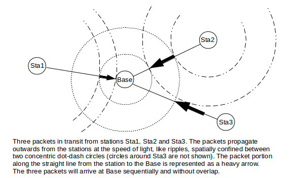
Because of the long distances involved, synchronization and transmission protocols must take account of speed-of-light delays. The round-trip delay across 30 km is 200 µsec which is ten times larger than the basic Wi-Fi SIFS interval; at 160 Mbps, this is the time needed to send 4 KB. If a station is to transmit so that its message arrives at the base station at a certain time, it must actually begin transmission early by an amount equal to the one-way station-to-base propagation delay; a special ranging mechanism allows stations to figure out this delay.
A subscriber station begins the network-entry connection process to a base station by listening for the base station’s transmissions (which may be organized into multiple channels); these message streams contain regular management messages containing, among other things, information about available data rates in each direction.
Also included in the base station’s message stream is information about start times for ranging intervals. The station waits for one of these intervals and sends a “range-request” message to the base station. These ranging intervals are open to all stations attempting network entry, and if another station transmits at the same time there will be a collision. However, network entry is only done once (for a given base station) and so the likelihood of a collision in any one ranging interval is small. An Ethernet/Wi-Fi-like exponential-backoff process is used if a collision does occur. Ranging intervals are the only times when collisions can occur; afterwards, all station transmissions are scheduled by the base station.
If there is no collision, the base station responds, and the station now knows the propagation delay and thus can determine when to transmit so that its data arrives at the base station exactly at a specified time. The station also determines its transmission signal strength from this ranging process.
Finally, and perhaps most importantly, the station receives from the base station its first timeslot for a scheduled transmission. These timeslot assignments are included in regular uplink-map packets broadcast by the base station. Each station’s timeslot includes both a start time and a total length; lengths are in the range of 2 to 20 ms. Future timeslots will be allocated as necessary by the base station, in future uplink-map packets. Scheduled timeslots may be periodic (as is would be appropriate for voice) or may occur at varying intervals. WiMAX stations may request any of several quality-of-service levels and the base station may take these requests into account when determining the schedule. The base station also creates a downlink schedule, but this does not need to be communicated to the subscriber stations; the base station simply uses it to decide what to broadcast when to the stations. When scheduling the timeslots, the base station may also take into account availability of multiple transmission channels and of directional antennas.
Through the uplink-map schedules and individual ranging, each station transmits so that one transmission finishes arriving just before the next transmission begins arriving, as seen from the perspective of the base station. Only minimal “guard intervals” need be included between consecutive transmissions. Two (or more) consecutive transmissions may in fact be “in the air” simultaneously, as far-away stations need to begin transmitting early so their signals will arrive at the base station at the expected time. The following diagram illustrates this for stations separated by relatively large physical distances.
Mobile stations will need to update their ranging information regularly, but this can be done through future scheduled transmissions. The distance to the base station is used not only for the mobile station’s transmission timing, but also to determine its power level; signals from each mobile station, no matter where located, should arrive at the base station with about the same power.
When a station has data to send, it includes in its next scheduled transmission a request for a longer transmission interval; if the request is granted, the station may send the data (or at least some of the data) in its next scheduled transmission slot. When a station is done transmitting, its timeslot shrinks to the minimum, and may be scheduled less frequently as well, but it does not disappear. Stations without data to send remain connected to the base station by sending “empty” messages during these slots.
3.5 Fixed Wireless
This category includes all wireless-service-provider systems where the subscriber’s location does not change. Often, but not always, the subscriber will have an outdoor antenna for improved reception and range. Fixed-wireless systems can involve relay through satellites, or can be terrestrial.
3.5.1 Terrestrial Wireless
For non-satellite systems, access points are usually tower-mounted and serve multiple subscribers, though point-to-point “microwave links” are also available. A multi-subscriber access point may serve an area with radius up to a hundred miles, depending on the technology. WiMAX 802.16d is one form of fixed wireless, but there are several others. Generally frequencies are 900 MHz and up, meaning that line-of-sight transmission is used. Frequencies may be either licensed or unlicensed. Some frequencies are better than others at “seeing” through trees and other obstructions.
Terrestrial fixed wireless was originally popularized for rural areas, where residential density is too low for economical cable connections. However, some fixed-wireless ISPs now operate in urban areas, often using WiMAX. One advantage of terrestrial fixed-wireless in remote areas is that the antennas covers a much smaller geographical area than a satellite, generally meaning that there is more data bandwidth available per user and the cost per megabyte is much lower.
Outdoor subscriber antennas often use a parabolic dish to improve reception; sizes range from 10 to 40 cm in diameter. The size of the dish may depend on the distance to the central tower.
While there are standardized fixed-wireless systems, such as WiMAX, there are also a number of proprietary alternatives, including systems from Trango and Canopy. Fixed-wireless systems might, in fact, be considered one of the last bastions of proprietary LAN protocols. This lack of standardization is due to a variety of factors; two primary ones are the relatively modest overall demand for this service and the the fact that most antennas need to be professionally installed by the ISP to ensure that they are “properly mounted, aligned, grounded and protected from lightning”.
3.5.2 Satellite Internet
An extreme case of fixed wireless is satellite Internet, in which signals pass through a satellite in geosynchronous orbit (35,786 km above the earth’s surface). Residential customers have parabolic antennas typically from 70 to 100 cm in diameter, larger than those used for terrestrial wireless but smaller than the dish antennas used at access points. Transmitter power is typically 1-2 watts, remarkably low for a signal that travels 35,786 km.
The primary problem associated with satellite Internet is very long RTTs. The the speed-of-light round-trip propagation delay is about 500 ms to which must be added queuing delays for the often-backlogged access point (my own personal experience suggested that RTTs of close to 1,000 ms were the norm). These long delays affect real-time traffic such as VoIP and gaming, but as we shall see in 14.11 The Satellite-Link TCP Problem bulk TCP transfers also perform poorly with very long RTTs. To provide partial compensation for the TCP issue, many satellite ISPs provide some sort of “acceleration” for bulk downloads: a web page, for example, would be downloaded rapidly by the access point and streamed to the satellite and back down to the user via a proprietary mechanism. Acceleration, however, cannot help interactive connections such as VPNs.
Another common feature of satellite Internet is a low daily utilization cap, typically in the hundreds of megabytes. Utilization caps are directly tied to the cost of maintaining satellites, but also to the fact that one satellite covers a great deal of ground, and so its available capacity is shared by a large number of users.
3.6 Token Ring
A significant part of the previous chapter was devoted to classic Ethernet’s collision mechanism for supporting shared media access. After that, it may come as a surprise that there is a simple multiple-access mechanism that is not only collision-free, but which supports fairness in the sense that if N stations wish to send then each will receive 1/N of the opportunities.
That method is Token Ring. Actual implementations come in several forms, from Fiber-Distributed Data Interface (FDDI) to so-called “IBM Token Ring”. The central idea is that stations are connected in a ring:
Packets will be transmitted in one direction (clockwise in the ring above). Stations in effect forward most packets around the ring, although they can also remove a packet. (It is perhaps more accurate to think of the forwarding as representing the default cable connectivity; non-forwarding represents the station’s momentarily breaking that connectivity.)
When the network is idle, all stations agree to forward a special, small packet known as a token. When a station, say A, wishes to transmit, it must first wait for the token to arrive at A. Instead of forwarding the token, A then transmits its own packet; this travels around the network and is then removed by A. At that point (or in some cases at the point when A finishes transmitting its data packet) A then forwards the token.
In a small ring network, the ring circumference may be a small fraction of one packet. Ring networks become “large” at the point when some packets may be entirely in transit on the ring. Slightly different solutions apply in each case. (It is also possible that the physical ring exists only within the token-ring switch, and that stations are connected to that switch using the usual point-to-point wiring.)
If all stations have packets to send, then we will have something like the following:
- A waits for the token
- A sends a packet
- A sends the token to B
- B sends a packet
- B sends the token to C
- C sends a packet
- C sends the token to D
- ...
All stations get an equal number of chances to transmit, and no bandwidth is wasted on collisions.
One problem with token ring is that when stations are powered off it is essential that the packets continue forwarding; this is usually addressed by having the default circuit configuration be to keep the loop closed. Another issue is that some station has to watch out in case the token disappears, or in case a duplicate token appears.
Because of fairness and the lack of collisions, IBM Token Ring was once considered to be the premium LAN mechanism. As such, a premium price was charged (there was also the matter of licensing fees). But due to a combination of lower hardware costs and higher bitrates (even taking collisions into account), Ethernet eventually won out.
There was also a much earlier collision-free hybrid of 10 Mbps Ethernet and Token Ring known as Token Bus: an Ethernet physical network (often linear) was used with a token-ring-like protocol layer above that. Stations were physically connected to the (linear) Ethernet but were assigned identifiers that logically arranged them in a (virtual) ring. Each station had to wait for the token and only then could transmit a packet; after that it would send the token on to the next station in the virtual ring. As with “real” Token Ring, some mechanisms need to be in place to monitor for token loss.
Token Bus Ethernet never caught on. The additional software complexity was no doubt part of the problem, but perhaps the real issue was that it was not necessary.
3.7 Virtual Circuits
Before we can get to our final LAN example, ATM, we need to detour briefly through virtual circuits.
Virtual circuits are The Road Not Taken by IP.
Virtual-circuit switching is an alternative to datagram switching, which was introduced in Chapter 1. In datagram switching, routers know the next_hop to each destination, and packets are addressed by destination. In virtual-circuit switching, routers know about end-to-end connections, and packets are “addressed” by a connection ID.
Before any packets can be sent, a connection needs to be established first. For that connection, the route is computed and then each link along the path is assigned a connection ID, traditionally called the VCI, for Virtual Circuit Identifier. In most cases, VCIs are only locally unique; that is, the same connection may use a different VCI on each link. The lack of global uniqueness makes VCI allocation much simpler. Although the VCI keeps changing along a path, the VCI can still be thought of as identifying the connection. To send a packet, the host marks the packet with the VCI assigned to the host–router1 link.
Packets arrive at (and depart from) switches via one of several ports, which we will assume are numbered beginning at 0. Switches maintain a connection table indexed by ⟨VCI,port⟩ pairs; unlike a forwarding table, the connection table has a record of every connection through that switch at that particular moment. As a packet arrives, its inbound VCIin and inbound portin are looked up in this table; this yields an outbound ⟨VCIout,portout⟩ pair. The VCI field of the packet is then rewritten to VCIout, and the packet is sent via portout.
Note that typically there is no source address information included in the packet (although the sender can be identified from the connection, which can be identified from the VCI at any point along the connection). Packets are identified by connection, not destination. Any node along the path (including the endpoints) can in principle look up the connection and figure out the endpoints.
Note also that each switch must rewrite the VCI. Datagram switches never rewrite addresses (though they do update hopcount/TTL fields). The advantage to this rewriting is that VCIs need be unique only for a given link, greatly simplifying the naming. Datagram switches also do not make use of a packet’s arrival interface.
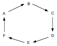
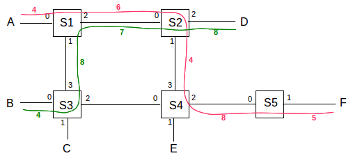
As an example, consider the network below. Switch ports are numbered 0,1,2,3. Two paths are drawn in, one from A to F in red and one from B to D in green; each link is labeled with its VCI number in the same color.
We will construct virtual-circuit connections between
- A and F (shown above in red)
- A and E
- A and C
- B and D (shown above in green)
- A and F again (a separate connection)
The following VCIs have been chosen for these connections. The choices are made more or less randomly here, but in accordance with the requirement that they be unique to each link. Because links are generally taken to be bidirectional, a VCI used from S1 to S3 cannot be reused from S3 to S1 until the first connection closes.
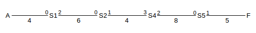
- A to F: A──4──S1──6──S2──4──S4──8──S5──5──F; this path goes from S1 to S4 via S2
- A to E: A──5──S1──6──S3──3──S4──8──E; this path goes, for no particular reason, from S1 to S4 via S3, the opposite corner of the square
- A to C: A──6──S1──7──S3──3──C
- B to D: B──4──S3──8──S1──7──S2──8──D
- A to F: A──7──S1──8──S2──5──S4──9──S5──2──F
One may verify that on any one link no two different paths use the same VCI.
We now construct the actual ⟨VCI,port⟩ tables for the switches S1-S4, from the above; the table for S5 is left as an exercise. Note that either the ⟨VCIin,portin⟩ or the ⟨VCIout,portout⟩ can be used as the key; we cannot have the same pair in both the in columns and the out columns. It may help to display the port numbers for each switch, as in the upper numbers in following diagram of the above red connection from A to F (lower numbers are the VCIs):
Switch S1:
| VCIin | portin | VCIout | portout | connection |
|---|---|---|---|---|
| 4 | 0 | 6 | 2 | A⟶F #1 |
| 5 | 0 | 6 | 1 | A⟶E |
| 6 | 0 | 7 | 1 | A⟶C |
| 8 | 1 | 7 | 2 | B⟶D |
| 7 | 0 | 8 | 2 | A⟶F #2 |
Switch S2:
| VCIin | portin | VCIout | portout | connection |
|---|---|---|---|---|
| 6 | 0 | 4 | 1 | A⟶F #1 |
| 7 | 0 | 8 | 2 | B⟶D |
| 8 | 0 | 5 | 1 | A⟶F #2 |
Switch S3:
| VCIin | portin | VCIout | portout | connection |
|---|---|---|---|---|
| 6 | 3 | 3 | 2 | A⟶E |
| 7 | 3 | 3 | 1 | A⟶C |
| 4 | 0 | 8 | 3 | B⟶D |
Switch S4:
| VCIin | portin | VCIout | portout | connection |
|---|---|---|---|---|
| 4 | 3 | 8 | 2 | A⟶F #1 |
| 3 | 0 | 8 | 1 | A⟶E |
| 5 | 3 | 9 | 2 | A⟶F #2 |
The namespace for VCIs is small, and compact (eg contiguous). Typically the VCI and port bitfields can be concatenated to produce a ⟨VCI,Port⟩ composite value small enough that it is suitable for use as an array index. VCIs work best as local identifiers. IP addresses, on the other hand, need to be globally unique, and thus are often rather sparsely distributed.
Virtual-circuit switching offers the following advantages:
- connections can get quality-of-service guarantees, because the switches are aware of connections and can reserve capacity at the time the connection is made
- headers are smaller, allowing faster throughput
- headers are small enough to allow efficient support for the very small packet sizes that are optimal for voice connections. ATM packets, for instance, have 48 bytes of data; see below.
Datagram forwarding, on the other hand, offers these advantages:
- Routers have less state information to manage.
- Router crashes and partial connection state loss are not a problem.
- If a router or link is disabled, rerouting is easy and does not affect any connection state. (As mentioned in Chapter 1, this was Paul Baran’s primary concern in his 1962 paper introducing packet switching.)
- Per-connection billing is very difficult.
The last point above may once have been quite important; in the era when the ARPANET was being developed, typical daytime long-distance rates were on the order of $1/minute. It is unlikely that early TCP/IP protocol development would have been as fertile as it was had participants needed to justify per-minute billing costs for every project.
It is certainly possible to do virtual-circuit switching with globally unique VCIs – say the concatenation of source and destination IP addresses and port numbers. The IP-based RSVP protocol (18.6 RSVP) does exactly this. However, the fast-lookup and small-header advantages of a compact namespace are then lost.
Note that virtual-circuit switching does not suffer from the problem of idle channels still consuming resources, which is an issue with circuits using time-division multiplexing (eg shared T1 lines)
3.8 Asynchronous Transfer Mode: ATM
ATM is a LAN mechanism intended to accommodate real-time traffic as well as bulk data transfer. It was particularly intended to support voice. A significant source of delay in voice traffic is the packet fill time: at DS0 speeds, a voice packet fills at 8 bytes/ms. If we are sending 1KB packets, this means voice is delayed by about 1/8 second, meaning in turn that when one person stops speaking, the earliest they can hear the other’s response is 1/4 second later. Voice delay also can introduce an annoying echo. When voice is sent over IP (VoIP), one common method is to send 160 bytes every 20 ms.
ATM took this small-packet strategy even further: packets have 48 bytes of data, plus 5 bytes of header. Such small packets are often called cells. To manage such a small header, virtual-circuit routing is a necessity. IP packets of such small size would likely consume more than 50% of the bandwidth on headers, if the LAN header were included.
Aside from reduced voice fill-time, other benefits to small cells are reduced store-and-forward delay and minimal queuing delay, at least for high-priority traffic. Prioritizing traffic and giving precedence to high-priority traffic is standard, but high-priority traffic is never allowed to interrupt transmission already begun of a low-priority packet. If you have a high-priority voice cell, and someone else has a 1500-byte packet just started, your cell has to wait about 30 cell times, because 1500 bytes is about 30 cells. However, if their low-priority traffic is instead made up of 30 cells, you have only to wait for their first cell to finish; the delay is 1/30 as much.
ATM also made the decision to require fixed-size cells. The penalty for one partially used cell among many is small. Having a fixed cell size simplifies hardware design, and, in theory, allows it easier to design for parallelism.
Unfortunately, ATM also chose to mandate no cell reordering. This means cells can use a smaller sequence-number field, but also makes parallel switches much harder to build. A typical parallel switch design might involve forwarding incoming cells to any of several input queues; the queues would then handle the VCI lookups in parallel and forward the cells to the appropriate output queues. With such an architecture, avoiding reordering is difficult. It is not clear to what extent the no-reordering decision was related to the later decline of ATM in the marketplace.
ATM cells have 48 bytes of data and a 5-byte header. The header contains up to 28 bits of VCI information, three “type” bits, one cell-loss priority, or CLP, bit, and an 8-bit checksum over the header only. The VCI is divided into 8-12 bits of Virtual Path Identifier and 16 bits of Virtual Channel Identifier, the latter supposedly for customer use to separate out multiple connections between two endpoints. Forwarding is by full switching only, and there is no mechanism for physical (LAN) broadcast.
3.8.1 ATM Segmentation and Reassembly
Due to the small packet size, ATM defines its own mechanisms for segmentation and reassembly of larger packets. Thus, individual ATM links in an IP network are quite practical. These mechanisms are called ATM Adaptation Layers, and there are four of them: AALs 1, 2, 3/4 and 5 (AAL 3 and AAL 4 were once separate layers, which merged). AALs 1 and 2 are used only for voice-type traffic; we will not consider them further.
The ATM segmentation-and-reassembly mechanism defined here is intended to apply only to large data; no cells are ever further subdivided. Furthermore, segmentation is always applied at the point where the data enters the network; reassembly is done at exit from the ATM path. IPv4 fragmentation, on the other hand, applies conceptually to IP packets, and may be performed by routers within the network.
For AAL 3/4, we first define a high-level “wrapper” for an IP packet, called the CS-PDU (Convergence Sublayer - Protocol Data Unit). This prefixes 32 bits on the front and another 32 bits (plus padding) on the rear. We then chop this into as many 44-byte chunks as are needed; each chunk goes into a 48-byte ATM payload, along with the following 32 bits worth of additional header/trailer:
- 2-bit type field:
- 10: begin new CS-PDU
- 00: continue CS-PDU
- 01: end of CS-PDU
- 11: single-segment CS-PDU
- 4-bit sequence number, 0-15, good for catching up to 15 dropped cells
- 10-bit MessageID field
- CRC-10 checksum.
We now have a total of 9 bytes of header for 44 bytes of data; this is more than 20% overhead. This did not sit well with the IP-over-ATM community (such as it was), and so AAL 5 was developed.
AAL 5 moved the checksum to the CS-PDU and increased it to 32 bits from 10 bits. The MID field was discarded, as no one used it, anyway (if you wanted to send several different types of messages, you simply created several virtual circuits). A bit from the ATM header was taken over and used to indicate:
- 1: start of new CS-PDU
- 0: continuation of an existing CS-PDU
The CS-PDU is now chopped into 48-byte chunks, which are then used as the entire body of each ATM cell. With 5 bytes of header for 48 bytes of data, overhead is down to 10%. Errors are detected by the CS-PDU CRC-32. This also detects lost cells (impossible with a per-cell CRC!), as we no longer have any cell sequence number.
For both AAL3/4 and AAL5, reassembly is simply a matter of stringing together consecutive cells in order of arrival, starting a new CS-PDU whenever the appropriate bits indicate this. For AAL3/4 the receiver has to strip off the 4-byte AAL3/4 headers; for AAL5 the receiver has to verify the CRC-32 checksum once all cells are received. Different cells from different virtual circuits can be jumbled together on the ATM “backbone”, but on any one virtual circuit the cells from one higher-level packet must be sent one right after the other.
A typical IP packet divides into about 20 cells. For AAL 3/4, this means a total of 200 bits devoted to CRC codes, versus only 32 bits for AAL 5. It might seem that AAL 3/4 would be more reliable because of this, but, paradoxically, it was not! The reason for this is that errors are rare, and so we typically have one or at most two per CS-PDU. Suppose we have only a single error, ie a single cluster of corrupted bits small enough that it is likely confined to a single cell. In AAL 3/4 the CRC-10 checksum will fail to detect that error (that is, the checksum of the corrupted packet will by chance happen to equal the checksum of the original packet) with probability 1/210. The AAL 5 CRC-32 checksum, however, will fail to detect the error with probability 1/232. Even if there are enough errors that two cells are corrupted, the two CRC-10s together will fail to detect the error with probability 1/220; the CRC-32 is better. AAL 3/4 is more reliable only when we have errors in at least four cells, at which point we might do better to switch to an error-correcting code.
Moral: one checksum over the entire message is often better than multiple shorter checksums over parts of the message.
3.9 Epilog
Along with a few niche protocols, we have focused primarily here on wireless and on virtual circuits. Wireless, of course, is enormously important: it is the enabler for mobile devices, and has largely replaced traditional Ethernet for home and office workstations.
While it is sometimes tempting (in the IP world at least) to write off ATM as a niche technology, virtual circuits are a serious conceptual alternative to datagram forwarding. As we shall see in 18 Quality of Service, IP has problems handling real-time traffic, and virtual circuits offer a solution. The Internet has so far embraced only small steps towards virtual circuits (such as MPLS, 18.12 Multi-Protocol Label Switching (MPLS)), but they remain a tantalizing strategy.
3.10 Exercises
1. Suppose remote host A uses a VPN connection to connect to host B, with IP address 200.0.0.7. A’s normal Internet connection is via device eth0 with IP address 12.1.2.3; A’s VPN connection is via device ppp0 with IP address 10.0.0.44. Whenever A wants to send a packet via ppp0, it is encapsulated and forwarded over the connection to B at 200.0.0.7.
2. Suppose remote host A wishes to use a TCP-based VPN connection to connect to host B, with IP address 200.0.0.7. However, the VPN software is not available for host A. Host A is, however, able to run that software on a virtual machine V hosted by A; A and V have respective IP addresses 10.0.0.1 and 10.0.0.2 on the virtual network connecting them. V reaches the outside world through network address translation (1.14 Network Address Translation), with A acting as V’s NAT router. When V runs the VPN software, it forwards packets addressed to B the usual way, through A using NAT. Traffic to any other destination it encapsulates over the VPN.
Can A configure its IP forwarding table so that it can make use of the VPN? If not, why not? If so, how? (If you prefer, you may assume V is a physical host connecting to a second interface on A; A still acts as V’s NAT router.)
3. Token Bus was a proprietary Ethernet-based network. It worked like Token Ring in that a small token packet was sent from one station to the next in agreed-upon order, and a station could transmit only when it had just received the token.
4. The IEEE 802.11 standard states “transmission of the ACK frame shall commence after a SIFS period, without regard to the busy/idle state of the medium”; that is, the ACK sender does not listen first for an idle network. Give a scenario in which the Wi-Fi ACK frame would fail to be delivered in the absence of this rule, but succeed with it. Hint: this is another example of the hidden-node problem.
5. Suppose the average backoff interval in a Wi-Fi network (802.11g) is 64 SlotTimes. The average packet size is 1 KB, and the data rate is 54 Mbps. At that data rate, it takes about (8×1000)/54 = 148 µsec to transmit a packet.
6. WiMAX subscriber stations are not expected to hear one another at all. For Wi-Fi non-access-point stations in an infrastructure (access-point) setting, on the other hand, listening to other non-access-point transmissions is encouraged.
7. Suppose WiMAX subscriber stations can be moving, at speeds of up to 33 meters/sec (the maximum allowed under 802.16e).
8. [SM90] contained a proposal for sending IP packets over ATM as N cells as in AAL-5, followed by one cell containing the XOR of all the previous cells. This way, the receiver can recover from the loss of any one cell. Suppose N=20 here; with the SM90 mechanism, each packet would require 21 cells to transmit; that is, we always send 5% more. Suppose the cell loss-rate is p (presumably very small). If we send 20 cells without the SM90 mechanism, we have a probability of about 20p that any one cell will be lost, and we will have to retransmit the entire 20 again. This gives an average retransmission amount of about 20p extra packets. For what value of p do the with-SM90 and the without-SM90 approaches involve about the same total number of cell transmissions?
9. In the example in 3.7 Virtual Circuits, give the VCI table for switch S5.
10. Suppose we have the following network:
A───S1────────S2───B
    │         │
    │         │
    │         │
C───S3────────S4───D
The virtual-circuit switching tables are below. Ports are identified by the node at the other end. Identify all the connections.
Switch S1:
| VCIin | portin | VCIout | portout |
|---|---|---|---|
| 1 | A | 2 | S3 |
| 2 | A | 2 | S2 |
| 3 | A | 3 | S2 |
Switch S2:
| VCIin | portin | VCIout | portout |
|---|---|---|---|
| 2 | S4 | 1 | B |
| 2 | S1 | 3 | S4 |
| 3 | S1 | 4 | S4 |
Switch S3:
| VCIin | portin | VCIout | portout |
|---|---|---|---|
| 2 | S1 | 2 | S4 |
| 3 | S4 | 2 | C |
Switch S4:
| VCIin | portin | VCIout | portout |
|---|---|---|---|
| 2 | S3 | 2 | S2 |
| 3 | S2 | 3 | S3 |
| 4 | S2 | 1 | D |
11. Suppose we have the following network:
A───S1────────S2───B
    │         │
    │         │
    │         │
C───S3────────S4───D
Give virtual-circuit switching tables for the following connections. Route via a shortest path.
12. Below is a set of switches S1 through S4. Define VCI-table entries so the virtual circuit from A to B follows the path
A ⟶ S1 ⟶ S2 ⟶ S4 ⟶ S3 ⟶ S1 ⟶ S2 ⟶ S4 ⟶ S3 ⟶ B
That is, each switch is visited twice.
A──S1─────S2
   │      │
   │      │
B──S3─────S4