2   Ethernet

We now turn to a deeper analysis of the ubiquitous Ethernet LAN protocol. Current user-level Ethernet today (2013) is usually 100 Mbps, with Gigabit Ethernet standard in server rooms and backbones, but because Ethernet speed scales in odd ways, we will start with the 10 Mbps formulation. While the 10 Mbps speed is obsolete, and while even the Ethernet collision mechanism is largely obsolete, collision management itself continues to play a significant role in wireless networks.

2.1   10-Mbps classic Ethernet

The original Ethernet specification was the 1976 paper of Metcalfe and Boggs, [MB76]. The data rate was 10 megabits per second, and all connections were made with coaxial cable instead of today’s twisted pair. In its original form, an Ethernet was a broadcast bus, which meant that all packets were, at least at the physical level, broadcast onto the shared medium and could be seen, theoretically, by all other nodes. If two nodes transmitted at the same time, there was a collision; proper handling of collisions was an important part of the access-mediation strategy for the shared medium. Data was transmitted using Manchester encoding; see 4.1.3   Manchester.

The linear bus structure could be modified with repeaters (below), into an arbitrary tree structure, though loops remain something of a problem even with today’s Ethernet.

Whenever two stations transmitted at the same time, the signals would collide, and interfere with one another; both transmissions would fail as a result. In order to minimize collision loss, each station implemented the following:

1. Before transmission, wait for the line to become quiet
2. While transmitting, continually monitor the line for signs that a collision has occurred; if a collision happens, then cease transmitting
3. If a collision occurs, use a backoff-and-retransmit strategy

These properties can be summarized with the CSMA/CD acronym: Carrier Sense, Multiple Access, Collision Detect. (The term “carrier sense” was used by Metcalfe and Boggs as a synonym for “signal sense”; there is no literal carrier frequency to be sensed.) It should be emphasized that collisions are a normal event in Ethernet, well-handled by the mechanisms above.

Classic Ethernet came in version 1 [1980, DEC-Intel-Xerox], version 2 [1982, DIX], and IEEE 802.3. There are some minor electrical differences between these, and one rather substantial packet-format difference. In addition to these, the Berkeley Unix trailing-headers packet format was used for a while.

There were three physical formats for 10 Mbps Ethernet cable: thick coax (10BASE-5), thin coax (10BASE-2), and, last to arrive, twisted pair (10BASE-T). Thick coax was the original; economics drove the successive development of the later two. The cheaper twisted-pair cabling eventually almost entirely displaced coax, at least for host connections.

The original specification included support for repeaters, which were in effect signal amplifiers although they might attempt to clean up a noisy signal. Repeaters processed each bit individually and did no buffering. In the telecom world, a repeater might be called a digital regenerator. A repeater with more than two ports was commonly called a hub; hubs allowed branching and thus much more complex topologies.

Bridges – later known as switches – came along a short time later. While repeaters act at the bit layer, a switch reads in and forwards an entire packet as a unit, and the destination address is likely consulted to determine to where the packet is forwarded. Originally, switches were seen as providing interconnection (“bridging”) between separate Ethernets, but later a switched Ethernet was seen as one large “virtual” Ethernet. We return to switching below in 2.4   Ethernet Switches.

Hubs propagate collisions; switches do not. If the signal representing a collision were to arrive at one port of a hub, it would, like any other signal, be retransmitted out all other ports. If a switch were to detect a collision one one port, no other ports would be involved; only packets received successfully are ever retransmitted out other ports.

In coaxial-cable installations, one long run of coax snaked around the computer room or suite of offices; each computer connected somewhere along the cable. Thin coax allowed the use of T-connectors to attach hosts; connections were made to thick coax via taps, often literally drilled into the coax central conductor. In a standalone installation one run of coax might be the entire Ethernet; otherwise, somewhere a repeater would be attached to allow connection to somewhere else.

Twisted-pair does not allow mid-cable attachment; it is only used for point-to-point links between hosts, switches and hubs. In a twisted-pair installation, each cable runs between the computer location and a central wiring closest (generally much more convenient than trying to snake coax all around the building). Originally each cable in the wiring closet plugged into a hub; nowadays the hub has likely been replaced by a switch.

There is still a role for hubs today when one wants to monitor the Ethernet signal from A to B (eg for intrusion detection analysis), although some switches now also support a form of monitoring.

All three cable formats could interconnect, although only through repeaters and hubs, and all used the same 10 Mbps transmission speed. While twisted-pair cable is still used by 100 Mbps Ethernet, it generally needs to be a higher-performance version known as Category 5, versus the 10 Mbps Category 3.

Here is the format of a typical Ethernet packet (DIX specification):

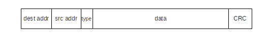
The destination and source addresses are 48-bit quantities; the type is 16 bits, the data length is variable up to a maximum of 1500 bytes, and the final CRC checksum is 32 bits. The checksum is added by the Ethernet hardware, never by the host software. There is also a preamble, not shown: a block of 1 bits followed by a 0, in the front of the packet, for synchronization. The type field identifies the next higher protocol layer; a few common type values are 0x0800 = IP, 0x8137 = IPX, 0x0806 = ARP.

The IEEE 802.3 specification replaced the type field by the length field, though this change never caught on. The two formats can be distinguished as long as the type values used are larger than the maximum Ethernet length of 1500 (or 0x05dc); the type values given in the previous paragraph all meet this condition.

Each Ethernet card has a (hopefully unique) physical address in ROM; by default any packet sent to this address will be received by the board and passed up to the host system. Packets addressed to other physical addresses will be seen by the card, but ignored (by default). All Ethernet devices also agree on a broadcast address of all 1’s: a packet sent to the broadcast address will be delivered to all attached hosts.

It is sometimes possible to change the physical address of a given card in software. It is almost universally possible to put a given card into promiscuous mode, meaning that all packets on the network, no matter what the destination address, are delivered to the attached host. This mode was originally intended for diagnostic purposes but became best known for the security breach it opens: it was once not unusual to find a host with network board in promiscuous mode and with a process collecting the first 100 bytes (presumably including userid and password) of every telnet connection.

2.1.1   Ethernet Multicast

Another category of Ethernet addresses is multicast, used to transmit to a set of stations; streaming video to multiple simultaneous viewers might use Ethernet multicast. The lowest-order bit in the first byte of an address indicates whether the address is physical or multicast. To receive packets addressed to a given multicast address, the host must inform its network interface that it wishes to do so; once this is done, any arriving packets addressed to that multicast address are forwarded to the host. The set of subscribers to a given multicast address may be called a multicast group. While higher-level protocols might prefer that the subscribing host also notifies some other host, eg the sender, this is not required, although that might be the easiest way to learn the multicast address involved. If several hosts subscribe to the same multicast address, then each will receive a copy of each multicast packet transmitted.

If switches (below) are involved, they must normally forward multicast packets on all outbound links, exactly as they do for broadcast packets; switches have no obvious way of telling where multicast subscribers might be. To avoid this, some switches do try to engage in some form of multicast filtering, sometimes by snooping on higher-layer multicast protocols. Multicast Ethernet is seldom used by IPv4, but plays a larger role in IPv6 configuration.

The second-to-lowest-order bit of the Ethernet address indicates, in the case of physical addresses, whether the address is believed to be globally unique or if it is only locally unique; this is known as the Universal/Local bit. When (global) Ethernet IDs are assigned by the manufacturer, the first three bytes serve to indicate the manufacturer. As long as the manufacturer involved is diligent in assigning the second three bytes, every manufacturer-provided Ethernet address should be globally unique. Lapses, however, are not unheard of.

2.1.2   The Slot Time and Collisions

The diameter of an Ethernet is the maximum distance between any pair of stations. The actual total length of cable can be much greater than this, if, for example, the topology is a “star” configuration. The maximum allowed diameter, measured in bits, is limited to 232 (a sample “budget” for this is below). This makes the round-trip-time 464 bits. As each station involved in a collision discovers it, it transmits a special jam signal of up to 48 bits. These 48 jam bits bring the total above to 512 bits, or 64 bytes. The time to send these 512 bits is the slot time of an Ethernet; time intervals on Ethernet are often described in bit times but in conventional time units the slot time is 51.2 µsec.

The value of the slot time determines several subsequent aspects of Ethernet. If a station has transmitted for one slot time, then no collision can occur (unless there is a hardware error) for the remainder of that packet. This is because one slot time is enough time for any other station to have realized that the first station has started transmitting, so after that time they will wait for the first station to finish. Thus, after one slot time a station is said to have acquired the network. The slot time is also used as the basic interval for retransmission scheduling, below.

Conversely, a collision can be received, in principle, at any point up until the end of the slot time. As a result, Ethernet has a minimum packet size, equal to the slot time, ie 64 bytes (or 46 bytes in the data portion). A station transmitting a packet this size is assured that if a collision were to occur, the sender would detect it (and be able to apply the retransmission algorithm, below). Smaller packets might collide and yet the sender not know it, ultimately leading to greatly reduced throughput.

If we need to send less than 46 bytes of data (for example, a 40-byte TCP ACK packet), the Ethernet packet must be padded out to the minimum length. As a result, all protocols running on top of Ethernet need to provide some way to specify the actual data length, as it cannot be inferred from the received packet size.

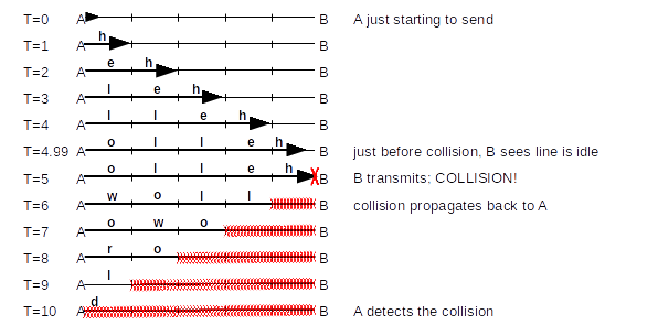
As a specific example of a collision occurring as late as possible, consider the diagram below. A and B are 5 units apart, and the bandwidth is 1 byte/unit. A begins sending “helloworld” at T=0; B starts sending just as A’s message arrives, at T=5. B has listened before transmitting, but A’s signal was not yet evident. A doesn’t discover the collision until 10 units have elapsed, which is twice the distance.

Here are typical maximum values for the delay in 10 Mbps Ethernet due to various components. These are taken from the Digital-Intel-Xerox (DIX) standard of 1982, except that “point-to-point link cable” is replaced by standard cable. The DIX specification allows 1500m of coax with two repeaters and 1000m of point-to-point cable; the table below shows 2500m of coax and four repeaters, following the later IEEE 802.3 Ethernet specification. Some of the more obscure delays have been eliminated. Entries are one-way delay times, in bits. The maximum path may have four repeaters, and ten transceivers (simple electronic devices between the coax cable and the NI cards), each with its drop cable (two transceivers per repeater, plus one at each endpoint).

Ethernet delay budget

item	length	delay, in bits	explanation (c = speed of light)
coax	2500M	110 bits	23 meters/bit (.77c)
transceiver cables	500M	25 bits	19.5 meters/bit (.65c)
transceivers		40 bits, max 10 units	4 bits each
repeaters		25 bits, max 4 units	6+ bits each (DIX 7.6.4.1)
encoders		20 bits, max 10 units	2 bits each (for signal generation)

The total here is 220 bits; in a full accounting it would be 232. Some of the numbers shown are a little high, but there are also signal rise time delays, sense delays, and timer delays that have been omitted. It works out fairly closely.

Implicit in the delay budget table above is the “length” of a bit. The speed of propagation in copper is about 0.77×c, where c=3×10⁸ m/sec = 300 m/µsec is the speed of light in vacuum. So, in 0.1 microseconds (the time to send one bit at 10 Mbps), the signal propagates approximately 0.77×c×10^-7 = 23 meters.

Ethernet packets also have a maximum packet size, of 1500 bytes. This limit is primarily for the sake of fairness, so one station cannot unduly monopolize the cable (and also so stations can reserve buffers guaranteed to hold an entire packet). At one time hardware vendors often marketed their own incompatible “extensions” to Ethernet which enlarged the maximum packet size to as much as 4KB. There is no technical reason, actually, not to do this, except compatibility.

The signal loss in any single segment of cable is limited to 8.5 db, or about 14% of original strength. Repeaters will restore the signal to its original strength. The reason for the per-segment length restriction is that Ethernet collision detection requires a strict limit on how much the remote signal can be allowed to lose strength. It is possible for a station to detect and reliably read very weak remote signals, but not at the same time that it is transmitting locally. This is exactly what must be done, though, for collision detection to work: remote signals must arrive with sufficient strength to be heard even while the receiving station is itself transmitting. The per-segment limit, then, has nothing to do with the overall length limit; the latter is set only to ensure that a sender is guaranteed of detecting a collision, even if it sends the minimum-sized packet.

2.1.3   Exponential Backoff Algorithm

Whenever there is a collision the exponential backoff algorithm is used to determine when each station will retry its transmission. Backoff here is called exponential because the range from which the backoff value is chosen is doubled after every successive collision involving the same packet. Here is the full Ethernet transmission algorithm, including backoff and retransmissions:

1. Listen before transmitting (“carrier detect”)
2. If line is busy, wait for sender to stop and then wait an additional 9.6 microseconds (96 bits). One consequence of this is that there is always a 96-bit gap between packets, so packets do not run together.
3. Transmit while simultaneously monitoring for collisions
4. If a collision does occur, send the jam signal, and choose a backoff time as follows: For transmission N, 1≤N≤10 (N=0 represents the original attempt), choose k randomly with 0 ≤ k < 2^N. Wait k slot times (k×51.2 µsec). Then check if the line is idle, waiting if necessary for someone else to finish, and then retry step 3. For 11≤N≤15, choose k randomly with 0 ≤ k < 1024 (= 2¹⁰)
5. If we reach N=16 (16 transmission attempts), give up.

If an Ethernet sender does not reach step 5, there is a very high probability that the packet was delivered successfully.

Exponential backoff means that if two hosts have waited for a third to finish and transmit simultaneously, and collide, then when N=1 they have a 50% chance of recollision; when N=2 there is a 25% chance, etc. When N≥10 the maximum wait is 52 milliseconds; without this cutoff the maximum wait at N=15 would be 1.5 seconds. As indicated above in the minimum-packet-size discussion, this retransmission strategy assumes that the sender is able to detect the collision while it is still sending, so it knows that the packet must be resent.

In the following diagram is an example of several stations attempting to transmit all at once, and using the above transmission/backoff algorithm to sort out who actually gets to acquire the channel. We assume we have five prospective senders A1, A2, A3, A4 and A5, all waiting for a sixth station to finish. We will assume that collision detection always takes one slot time (it will take much less for nodes closer together) and that the slot start-times for each station are synchronized; this allows us to measure time in slots. A solid arrow at the start of a slot means that sender began transmission in that slot; a red X signifies a collision. If a collision occurs, the backoff value k is shown underneath. A dashed line shows the station waiting k slots for its next attempt.

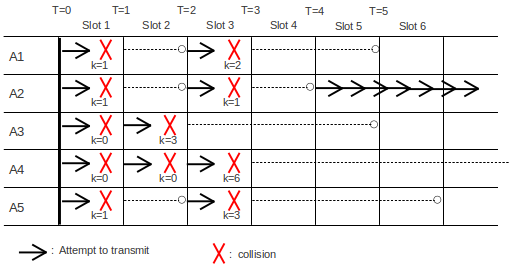
At T=0 we assume the transmitting station finishes, and all the Ai transmit and collide. At T=1, then, each of the Ai has discovered the collision; each chooses a random k<2. Let us assume that A1 chooses k=1, A2 chooses k=1, A3 chooses k=0, A4 chooses k=0, and A5 chooses k=1.

Those stations choosing k=0 will retransmit immediately, at T=1. This means A3 and A4 collide again, and at T=2 they now choose random k<4. We will Assume A3 chooses k=3 and A4 chooses k=0; A3 will try again at T=2+3=5 while A4 will try again at T=2, that is, now.

At T=2, we now have the original A1, A2, and A5 transmitting for the second time, while A4 trying again for the third time. They collide. Let us suppose A1 chooses k=2, A2 chooses k=1, A5 chooses k=3, and A4 chooses k=6 (A4 is choosing k<8 at random). Their scheduled transmission attempt times are now A1 at T=3+2=5, A2 at T=4, A5 at T=6, and A4 at T=9.

At T=3, nobody attempts to transmit. But at T=4, A2 is the only station to transmit, and so successfully seizes the channel. By the time T=5 rolls around, A1 and A3 will check the channel, that is, listen first, and wait for A2 to finish. At T=9, A4 will check the channel again, and also begin waiting for A2 to finish.

A maximum of 1024 hosts is allowed on an Ethernet. This number apparently comes from the maximum range for the backoff time as 0 ≤ k < 1024. If there are 1024 hosts simultaneously trying to send, then, once the backoff range has reached k<1024 (N=10), we have a good chance that one station will succeed in seizing the channel, that is; the minimum value of all the random k’s chosen will be unique.

This backoff algorithm is not “fair”, in the sense that the longer a station has been waiting to send, the lower its priority sinks. Newly transmitting stations with N=0 need not delay at all. The Ethernet capture effect, below, illustrates this unfairness.

2.1.4   Capture effect

The capture effect is a scenario illustrating the potential lack of fairness in the exponential backoff algorithm. The unswitched Ethernet must be fully busy, in that each of two senders always has a packet ready to transmit.

Let A and B be two such busy nodes, simultaneously starting to transmit their first packets. They collide. Suppose A wins, and sends. When A is finished, B tries to transmit again. But A has a second packet, and so A tries too. A chooses a backoff k<2 (that is, between 0 and 1 inclusive), but since B is on its second attempt it must choose k<4. This means A is favored to win. Suppose it does.

After that transmission is finished, A and B try yet again: A on its first attempt for its third packet, and B on its third attempt for its first packet. Now A again chooses k<2 but B must choose k<8; this time A is much more likely to win. Each time B fails to win a given backoff, its probability of winning the next one is reduced by about 1/2. It is quite possible, and does occur in practice, for B to lose all the backoffs until it reaches the maximum of N=16 attempts; once it has lost the first three or four this is in fact quite likely. At this point B simply discards the packet and goes on to the next one with N reset to 1 and k chosen from {0,1}.

The capture effect can be fixed with appropriate modification of the backoff algorithm; the Binary Logarithmic Arbitration Method (BLAM) was proposed in [MM94]. The BLAM algorithm was considered for the then-nascent 100 Mbps “Fast” Ethernet standard. But in the end a hardware strategy won out: Fast Ethernet supports “full-duplex” mode which is collision-free (see 2.2   100 Mbps (Fast) Ethernet, below). While full-duplex mode is not required for using Fast Ethernet, it was assumed that any sites concerned enough about performance to be worried about the capture effect would opt for full-duplex.

2.1.5   Hubs and topology

Ethernet hubs (multiport repeaters) change the topology, but not the fundamental constraints. Hubs allow much more branching; typically, each station in the office now has its own link to the wiring closet. Loops are still forbidden. Before inexpensive switches were widely available, 10BASE-T (twisted pair Ethernet) used hubs heavily; with twisted pair, a device can only connect to the endpoint of the wire. Thus, typically, each host is connected directly to a hub. The maximum diameter of an Ethernet consisting of multiple segments, joined by hubs, is constrained by the round-trip-time, and the need to detect collisions before the sender has completed sending, as before. However, twisted-pair links are required to be much shorter, about 100 meters.

2.1.6   Errors

Packets can have bits flipped or garbled by electrical noise on the cable; estimates of the frequency with which this occurs range from 1 in 10⁴ to 1 in 10⁶. Bit errors are not uniformly likely; when they occur, they are likely to occur in bursts. Packets can also be lost in hubs, although this appears less likely. Packets can be lost due to collisions only if the sending host makes 16 unsuccessful transmission attempts and gives up. Ethernet packets contain a 32-bit CRC error-detecting code (see 5.4.1   Cyclical Redundancy Check: CRC) to detect bit errors. Packets can also be misaddressed by the sending host, or, most likely of all, they can arrive at the receiving host at a point when the receiver has no free buffers and thus be dropped by a higher-layer protocol.

2.1.7   CSMA persistence

A carrier-sense/multiple-access transmission strategy is said to be nonpersistent if, when the line is busy, the sender waits a randomly selected time. A strategy is p-persistent if, after waiting for the line to clear, the sender sends with probability p≤1. Ethernet uses 1-persistence. A consequence of 1-persistence is that, if more than one station is waiting for line to clear, then when the line does clear a collision is certain. However, Ethernet then gracefully handles the resulting collision via the usual exponential backoff. If N stations are waiting to transmit, the time required for one station to win the backoff is linear in N.

When we consider the Wi-Fi collision-handling mechanisms in 3.3   Wi-Fi, we will see that collisions cannot be handled quite as cheaply: for one thing, there is no way to detect a collision in progress, so the entire packet-transmission time is wasted. In the Wi-Fi case, p-persistence is used with p<1.

An Ethernet broadcast storm was said to occur when there were too many transmission attempts, and most of the available bandwidth was tied up in collisions. A properly functioning classic Ethernet had an effective bandwidth of as much as 50-80% of the nominal 10Mbps capacity, but attempts to transmit more than this typically resulted in successfully transmitting a good deal less.

2.1.8   Analysis of Classic Ethernet

How much time does Ethernet “waste” on collisions? A paradoxical attribute of Ethernet is that raising the transmission-attempt rate on a busy segment can reduce the actual throughput. More transmission attempts can lead to longer contention intervals between packets, as senders use the transmission backoff algorithm to attempt to acquire the channel. What effective throughput can be achieved?

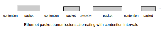
It is convenient to refer to the time between packet transmissions as the contention interval even if there is no actual contention, even if the network is idle. Thus, a timeline for Ethernet always consists of alternating packet transmissions and contention intervals:

As a first look at contention intervals, assume that there are N stations waiting to transmit at the start of the interval. It turns out that, if all follow the exponential backoff algorithm, we can expect O(N) slot times before one station successfully acquires the channel; thus, Ethernets are happiest when N is small and there are only a few stations simultaneously transmitting. However, multiple stations are not necessarily a severe problem. Often the number of slot times needed turns out to be about N/2, and slot times are short. If N=20, then N/2 is 10 slot times, or 640 bytes. However, one packet time might be 1500 bytes. If packet intervals are 1500 bytes and contention intervals are 640 byes, this gives an overall throughput of 1500/(640+1500) = 70% of capacity. In practice, this seems to be a reasonable upper limit for the throughput of classic shared-media Ethernet.

2.1.8.1   The ALOHA models

We get very similar throughput values when we analyze the Ethernet contention interval using the ALOHA model that was a precursor to Ethernet, and assume a very large number of active senders, each transmitting at a very low rate.

In the ALOHA model, stations transmit packets without listening first for a quiet line or monitoring the transmission for collisions (this models the situation of several ground stations transmitting to a satellite; the ground stations are presumed unable to see one another). To model the success rate of ALOHA, assume all the packets are the same size and let T be the time to send one (fixed-size) packet; T represents the Aloha slot time. We will find the transmission rate that optimizes throughput.

The core assumption of this model is that that a large number N of hosts are transmitting, each at a relatively low rate of s packets/slot. Denote by G the average number of transmission attempts per slot; we then have G = Ns. We will derive an expression for S, the average rate of successful transmissions per slot, in terms of G.

If two packets overlap during transmissions, both are lost. Thus, a successful transmission requires everyone else quiet for an interval of 2T: if a sender succeeds in the interval from t to t+T, then no other node can have tried to begin transmission in the interval t−T to t+T. The probability of one station transmitting during an interval of time T is G = Ns; the probability of the remaining N−1 stations all quiet for an interval of 2T is (1−s)^2(N−1). The probability of a successful transmission is thus

S = Ns*(1−s)^2(N−1)

= G(1−G/N)^2N

⟶ Ge^-2G as N⟶∞.

The function S = G e^-2G has a maximum at G=1/2, S=1/2e. The rate G=1/2 means that, on average, a transmission is attempted every other slot; this yields the maximum successful-transmission throughput of 1/2e. In other words, at this maximum attempt rate G=1/2, we expect about 2e−1 slot times worth of contention between successful transmissions. What happens to the remaining G−S unsuccessful attempts is not addressed by this model; presumably some higher-level mechanism (eg backoff) leads to retransmissions.

A given throughput S<1/2e may be achieved at either of two values for G; that is, a given success rate may be due to a comparable attempt rate or else due to a very high attempt rate with a similarly high failure rate.

2.1.8.2   ALOHA and Ethernet

The relevance of the Aloha model to Ethernet is that during one Ethernet slot time there is no way to detect collisions (they haven’t reached the sender yet!) and so the Ethernet contention phase resembles ALOHA with an Aloha slot time T of 51.2 microseconds. Once an Ethernet sender succeeds, however, it continues with a full packet transmission, which is presumably many times longer than T.

The average length of the contention interval, at the maximum throughput calculated above, is 2e−1 slot times (from ALOHA); recall that our model here supposed many senders sending at very low individual rates. This is the minimum contention interval; with lower loads the contention interval is longer due to greater idle times and with higher loads the contention interval is longer due to more collisions.

Finally, let P be the time to send an entire packet in units of T; ie the average packet size in units of T. P is thus the length of the “packet” phase in the diagram above. The contention phase has length 2e−1, so the total time to send one packet (contention+packet time) is 2e−1+P. The useful fraction of this is, of course, P, so the effective maximum throughput is P/(2e−1+P).

At 10Mbps, T=51.2 microseconds is 512 bits, or 64 bytes. For P=128 bytes = 2*64, the effective bandwidth becomes 2/(2e-1+2), or 31%. For P=512 bytes=8*64, the effective bandwidth is 8/(2e+7), or 64%. For P=1500 bytes, the model here calculates an effective bandwidth of 80%.

These numbers are quite similar to our earlier values based on a small number of stations sending constantly.

2.2   100 Mbps (Fast) Ethernet

In all the analysis here of 10 Mbps Ethernet, what happens when the bandwidth is increased to 100 Mbps, as is done in the so-called Fast Ethernet standard? If the network physical diameter remains the same, then the round-trip time will be the same in microseconds but will be 10-fold larger measured in bits; this might mean a minimum packet size of 640 bytes instead of 64 bytes. (Actually, the minimum packet size might be somewhat smaller, partly because the “jam signal” doesn’t have to speed up at all, and partly because some of the numbers in the 10 Mbps delay budget above were larger than necessary, but it would still be large enough that a substantial amount of bandwidth would be consumed by padding.) The designers of Fast Ethernet felt this was impractical.

However, Fast Ethernet was developed at a time (~1995) when reliable switches (below) were widely available, and “longer” networks could be formed by chaining together shorter ones with switches. So instead of increasing the minimum packet size, the decision was made to ensure collision detectability by reducing the network diameter instead. The network diameter chosen was a little over 400 meters, with reductions to account for the presence of hubs. At 2.3 meters/bit, 400 meters is 174 bits, for a round-trip of 350 bits.

This 400-meter number, however, may be misleading: by far the most popular Fast Ethernet standard is 100BASE-TX which uses twisted-pair copper wire (so-called Category 5, or better), and in which any individual cable segment is limited to 100 meters. The maximum 100BASE-TX network diameter – allowing for hubs – is just over 200 meters. The 400-meter distance does apply to optical-fiber-based 100BASE-FX in half-duplex mode, but this is not common.

The 100BASE-TX network-diameter limit of 200 meters might seem small; it amounts in many cases to a single hub with multiple 100-meter cable segments radiating from it. In practice, however, such “star” configurations can easily be joined with switches. As we will see below in 2.4   Ethernet Switches, switches partition an Ethernet into separate “collision domains”; the network-diameter rules apply to each domain separately but not to the aggregated whole. In a fully switched (that is, no hubs) 100BASE-TX LAN, each collision domain is simply a single twisted-pair link, subject to the 100-meter maximum length.

Fast Ethernet also introduced the concept of full-duplex Ethernet: two twisted pairs could be used, one for each direction. Full-duplex Ethernet is limited to paths not involving hubs, that is, to single station-to-station links, where a station is either a host or a switch. Because such a link has only two potential senders, and each sender has its own transmit line, full-duplex Ethernet is collision-free.

Fast Ethernet uses 4B/5B encoding, covered in 4.1.4   4B/5B.

Fast Ethernet 100BASE-TX does not particularly support links between buildings, due to the network-diameter limitation. However, fiber-optic point-to-point links are quite effective here, provided full-duplex is used to avoid collisions. We mentioned above that the coax-based 100BASE-FX standard allowed a maximum half-duplex run of 400 meters, but 100BASE-FX is much more likely to use full duplex, where the maximum cable length rises to 2,000 meters.

2.3   Gigabit Ethernet

If we continue to maintain the same slot time but raise the transmission rate to 1000 Mbps, the network diameter would now be 20-40 meters. Instead of that, Gigabit Ethernet moved to a 4096-bit (512-byte) slot time, at least for the twisted-pair versions. Short frames need to be padded, but this padding is done by the hardware. Gigabit Ethernet 1000Base-T uses so-called PAM-5 encoding, below, which supports a special pad pattern (or symbol) that cannot appear in the data. The hardware pads the frame with these special patterns, and the receiver can thus infer the unpadded length as set by the host operating system.

However, the Gigabit Ethernet slot time is largely irrelevant, as full-duplex (bidirectional) operation is almost always supported. Combined with the restriction that each length of cable is a station-to-station link (that is, hubs are no longer allowed), this means that collisions simply do not occur and the network diameter is no longer a concern.

There are actually multiple Gigabit Ethernet standards (as there are for Fast Ethernet). The different standards apply to different cabling situations. There are full-duplex optical-fiber formulations good for many miles (eg 1000Base-LX10), and even a version with a 25-meter maximum cable length (1000Base-CX), which would in theory make the original 512-bit slot practical.

The most common gigabit Ethernet over copper wire is 1000BASE-T (sometimes incorrectly referred to as 100BASE-TX. While there exists a TX, it requires Category 6 cable and is thus seldom used; many devices labeled TX are in fact 1000BASE-T). For 1000BASE-T, all four twisted pairs in the cable are used. Each pair transmits at 250 Mbps, and each pair is bidirectional, thus supporting full-duplex communication. Bidirectional communication on a single wire pair takes some careful echo cancellation at each end, using a circuit known as a “hybrid” that in effect allows detection of the incoming signal by filtering out the outbound signal.

On any one cable pair, there are five signaling levels. These are used to transmit two-bit symbols (4.1.4   4B/5B) at a rate of 125 symbols/µsec, for a data rate of 250 bits/µsec. Two-bit symbols in theory only require four signaling levels; the fifth symbol allows for some redundancy which is used for error detection and correction, for avoiding long runs of identical symbols, and for supporting a special pad symbol, as mentioned above. The encoding is known as 5-level pulse-amplitude modulation, or PAM-5. The target bit error rate (BER) for 1000BASE-T is 10^-10, meaning that the packet error rate is less than 1 in 10⁶.

In developing faster Ethernet speeds, economics plays at least as important a role as technology. As new speeds reach the market, the earliest adopters often must take pains to buy cards, switches and cable known to “work together”; this in effect amounts to installing a proprietary LAN. The real benefit of Ethernet, however, is arguably that it is standardized, at least eventually, and thus a site can mix and match its cards and devices. Having a given Ethernet standard support existing cable is even more important economically; the costs of replacing cable often dwarf the costs of the electronics.

2.4   Ethernet Switches

Switches join separate physical Ethernets (or Ethernets and token rings). A switch has two or more Ethernet interfaces; when a packet is received on one interface it is retransmitted on one or more other interfaces. Only valid packets are forwarded; collisions are not propagated. The term collision domain is sometimes used to describe the region of an Ethernet in between switches; a given collision propagates only within its collision domain. All the collision-detection rules, including the rules for maximum network diameter, apply only to collision domains, and not to the larger “virtual Ethernets” created by stringing collision domains together with switches.

As we shall see below, a switched Ethernet offers much more resistance to eavesdropping than a non-switched (eg hub-based) Ethernet.

Like simpler unswitched Ethernets, the topology for a switched Ethernet is in principle required to be loop-free, although in practice, most switches support the spanning-tree loop-detection protocol and algorithm, below, which automatically “prunes” the network topology to make it loop-free.

And while a switch does not propagate collisions, it must maintain a queue for each outbound interface in case it needs to forward a packet at a moment when the interface is busy; on occasion packets are lost when this queue overflows.

Ethernet switches use datagram forwarding as described in 1.4   Datagram Forwarding. They start out with empty forwarding tables, and build them through a “learning” process. If a switch does not have an entry for a particular destination, it will fall back on broadcast: it will forward the packet out every interface other than the one on which the packet arrived.

A switch learns address locations as follows: for each interface, the switch maintains a table of physical addresses that have appeared as source addresses in packets arriving via that interface. The switch thus knows that to reach these addresses, if one of them later shows up as a destination address, the packet needs to be sent only via that interface. Specifically, when a packet arrives on interface I with source address S and destination unicast address D, the switch enters ⟨S,I⟩ into its forwarding table.

To actually deliver the packet, the switch also looks up D in the forwarding table. If there is an entry ⟨D,J⟩ with J≠I – that is, D is known to be reached via interface J – then the switch forwards the packet out interface J. If J=I, that is, the packet has arrived on the same interfaces by which the destination is reached, then the packet does not get forwarded at all; it presumably arrived at interface I only because that interface was connected to a shared Ethernet segment that also either contained D or contained another switch that would bring the packet closer to D. If there is no entry for D, the switch must forward the packet out all interfaces J with J≠I; this represents the fallback to broadcast. As time goes on, this fallback to broadcast is needed less and less often.

If the destination address D is the broadcast address, or, for many switches, a multicast address, broadcast is required.

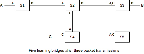
In the diagram above, each switch’s tables are indicated by listing near each interface the destinations known to be reachable by that interface. The entries shown are the result of the following packets:

• A sends to B; all switches learn where A is
• B sends to A; this packet goes directly to A; only S3, S2 and S1 learn where B is
• C sends to B; S4 does not know where B is so this packet goes to S5; S2 does know where B is so the packet does not go to S1.

Once all the switches have learned where all (or most of) the hosts are, packet routing becomes optimal. At this point packets are never sent on links unnecessarily; a packet from A to B only travels those links that lie along the (unique) path from A to B. (Paths must be unique because switched Ethernet networks cannot have loops, at least not active ones. If a loop existed, then a packet sent to an unknown destination would be forwarded around the loop endlessly.)

Switches have an additional advantage in that traffic that does not flow where it does not need to flow is much harder to eavesdrop on. On an unswitched Ethernet, one host configured to receive all packets can eavesdrop on all traffic. Early Ethernets were notorious for allowing one unscrupulous station to capture, for instance, all passwords in use on the network. On a fully switched Ethernet, a host physically only sees the traffic actually addressed to it; other traffic remains inaccessible.

Typical switches have room for table with 10⁴ - 10⁶ entries, though maxing out at 10⁵ entries may be more common; this is usually enough to learn about all hosts in even a relatively large organization. A switched Ethernet can fail when total traffic becomes excessive, but excessive total traffic would drown any network (although other network mechanisms might support higher bandwidth). The main limitations specific to switching are the requirement that the topology must be loop-free (thus disallowing duplicate paths which might otherwise provide redundancy), and that all broadcast traffic must always be forwarded everywhere. As a switched Ethernet grows, broadcast traffic comprises a larger and larger percentage of the total traffic, and the organization must at some point move to a routing architecture (eg as in 7.6   IP Subnets).

One of the differences between an inexpensive Ethernet switch and a pricier one is the degree of internal parallelism it can support. If three packets arrive simultaneously on ports 1, 2 and 3, and are destined for respective ports 4, 5 and 6, can the switch actually transmit the packets simultaneously? A simple switch likely has a single CPU and a single memory bus, both of which can introduce transmission bottlenecks. For commodity five-port switches, at most two simultaneous transmissions can occur; such switches can generally handle that degree of parallelism. It becomes harder as the number of ports increases, but at some point the need to support full parallel operation can be questioned; in many settings the majority of traffic involves one or two server or router ports. If a high degree of parallelism is in fact required, there are various architectures – known as switch fabrics – that can be used; these typically involve multiple simple processor elements.

2.5   Spanning Tree Algorithm

In theory, if you form a loop with Ethernet switches, any packet with destination not already present in the forwarding tables will circulate endlessly; naive switches will actually do this.

In practice, however, loops allow a form of redundancy – if one link breaks there is still 100% connectivity – and so are desirable. As a result, Ethernet switches have incorporated a switch-to-switch protocol to construct a subset of the switch-connections graph that has no loops and yet allows reachability of every host, known as a spanning tree. The switch-connections graph is the graph with nodes consisting of both switches and of the unswitched Ethernet segments and isolated individual hosts connected to the switches. Multi-host Ethernet segments are most often created via Ethernet hubs (repeaters). Edges in the graph represent switch-segment and switch-switch connections; each edge attaches to its switch via a particular, numbered interface. The goal is to disable redundant (cyclical) paths while remaining able to deliver to any segment. The algorithm is due to Radia Perlman, [RP85].

Once the spanning tree is built, all packets are sent only via edges in the tree, which, as a tree, has no loops. Switch ports (that is, edges) that are not part of the tree are not used at all, even if they would represent the most efficient path for that particular destination. If a given segment connects to two switches that both connect to the root node, the switch with the shorter path to the root is used, if possible; in the event of ties, the switch with the smaller ID is used. The simplest measure of path cost is the number of hops, though current implementations generally use a cost factor inversely proportional to the bandwidth (so larger bandwidth has lower cost). Some switches permit other configuration here. The process is dynamic, so if an outage occurs then the spanning tree is recomputed. If the outage should partition the network into two pieces, both pieces will build spanning trees.

All switches send out regular messages on all interfaces called bridge protocol data units, or BPDUs (or “Hello” messages). These are sent to the Ethernet multicast address 01:80:c2:00:00:00, from the Ethernet physical address of the interface. (Note that Ethernet switches do not otherwise need a unique physical address for each interface.) The BPDUs contain

• The switch ID
• the ID of the node the switch believes is the root
• the path cost to that root

These messages are recognized by switches and are not forwarded naively. Bridges process each message, looking for

• a switch with a lower ID (thus becoming the new root)
• a shorter path to the existing root
• an equal-length path to the existing root, but via a switch or port with a lower ID (the tie-breaker rule)

When a switch sees a new root candidate, it sends BPDUs on all interfaces, indicating the distance. The switch includes the interface leading towards the root.

Once this process is complete, each switch knows

• its own path to the root
• which of its ports any further-out switches will be using to reach the root
• for each port, its directly connected neighboring switches

Now the switch can “prune” some (or all!) of its interfaces. It disables all interfaces that are not enabled by the following rules:

1. It enables the port via which it reaches the root
2. It enables any of its ports that further-out switches use to reach the root
3. If a remaining port connects to a segment to which other “segment-neighbor” switches connect as well, the port is enabled if the switch has the minimum cost to the root among those segment-neighbors, or, if a tie, the smallest ID among those neighbors, or, if two ports are tied, the port with the smaller ID.
4. If a port has no directly connected switch-neighbors, it presumably connects to a host or segment, and the port is enabled.

Rules 1 and 2 construct the spanning tree; if S3 reaches the root via S2, then Rule 1 makes sure S3’s port towards S2 is open, and Rule 2 makes sure S2’s corresponding port towards S3 is open. Rule 3 ensures that each network segment that connects to multiple switches gets a unique path to the root: if S2 and S3 are segment-neighbors each connected to segment N, then S2 enables its port to N and S3 does not (because 2<3). The primary concern here is to create a path for any host nodes on segment N; S2 and S3 will create their own paths via Rules 1 and 2. Rule 4 ensures that any “stub” segments retain connectivity; these would include all hosts directly connected to switch ports.

2.5.1   Example 1: Switches Only

We can simplify the situation somewhat if we assume that the network is fully switched: each switch port connects to another switch or to a (single-interface) host; that is, no repeater hubs (or coax segments!) are in use. In this case we can dispense with Rule 3 entirely.

Any switch ports directly connected to a host can be identified because they are “silent”; the switch never receives any BPDU messages on these interfaces because hosts do not send these. All these host port ends up enabled via Rule 4. Here is our sample network, where the switch numbers (eg 5 for S5) represent their IDs; no hosts are shown and interface numbers are omitted.

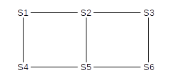
S1 has the lowest ID, and so becomes the root. S2 and S4 are directly connected, so they will enable the interfaces by which they reach S1 (Rule 1) while S1 will enable its interfaces by which S2 and S4 reach it (Rule 2).

S3 has a unique lowest-cost route to S1, and so again by Rule 1 it will enable its interface to S2, while by Rule 2 S2 will enable its interface to S3.

S5 has two choices; it hears of equal-cost paths to the root from both S2 and S4. It picks the lower-numbered neighbor S2; the interface to S4 will never be enabled. Similarly, S4 will never enable its interface to S5.

Similarly, S6 has two choices; it selects S3.

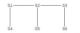
After these links are enabled (strictly speaking it is interfaces that are enabled, not links, but in all cases here either both interfaces of a link will be enabled or neither), the network in effect becomes:

2.5.2   Example 2: Switches and Segments

As an example involving switches that may join via unswitched Ethernet segments, consider the following network; S1, S2 and S3, for example, are all segment-neighbors via their common segment B. As before, the switch numbers represent their IDs. The letters in the clouds represent network segments; these clouds may include multiple hosts. Note that switches have no way to detect these hosts; only (as above) other switches.

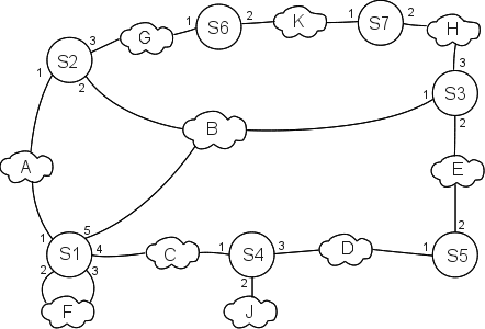
Eventually, all switches discover S1 is the root (because 1 is the smallest of {1,2,3,4,5,6}). S2, S3 and S4 are one (unique) hop away; S5, S6 and S7 are two hops away.

Algorhyme

I think that I shall never see

a graph more lovely than a tree.

A tree whose crucial property

is loop-free connectivity.

A tree that must be sure to span

so packet can reach every LAN.

First, the root must be selected.

By ID, it is elected.

Least-cost paths from root are traced.

In the tree, these paths are placed.

A mesh is made by folks like me,

then bridges find a spanning tree.

Radia Perlman

For the switches one hop from the root, Rule 1 enables S2’s port 1, S3’s port 1, and S4’s port 1. Rule 2 enables the corresponding ports on S1: ports 1, 5 and 4 respectively. Without the spanning-tree algorithm S2 could reach S1 via port 2 as well as port 1, but port 1 has a smaller number.

S5 has two equal-cost paths to the root: S5⟶S4⟶S1 and S5⟶S3⟶S1. S3 is the switch with the lower ID; its port 2 is enabled and S5 port 2 is enabled.

S6 and S7 reach the root through S2 and S3 respectively; we enable S6 port 1, S2 port 3, S7 port 2 and S3 port 3.

The ports still disabled at this point are S1 ports 2 and 3, S2 port 2, S4 ports 2 and 3, S5 port 1, S6 port 2 and S7 port 1.

Now we get to Rule 3, dealing with how segments (and thus their hosts) connect to the root. Applying Rule 3,

• We do not enable S2 port 2, because the network (B) has a direct connection to the root, S1
• We do enable S4 port 3, because S4 and S5 connect that way and S4 is closer to the root. This enables connectivity of network D. We do not enable S5 port 1.
• S6 and S7 are tied for the path-length to the root. But S6 has smaller ID, so it enables port 2. S7’s port 1 is not enabled.

Finally, Rule 4 enables S4 port 2, and thus connectivity for host J. It also enables S1 port 2; network F has two connections to S1 and port 2 is the lower-numbered connection.

All this port-enabling is done using only the data collected during the root-discovery phase; there is no additional negotiation. The BPDU exchanges continue, however, so as to detect any changes in the topology.

If a link is disabled, it is not used even in cases where it would be more efficient to use it. That is, traffic from F to B is sent via B1, D, and B5; it never goes through B7. IP routing, on the other hand, uses the “shortest path”. To put it another way, all spanning-tree Ethernet traffic goes through the root node, or along a path to or from the root node.

The traditional (IEEE 802.1D) spanning-tree protocol is relatively slow; the need to go through the tree-building phase means that after switches are first turned on no normal traffic can be forwarded for ~30 seconds. Faster, revised protocols have been proposed to reduce this problem.

Another issue with the spanning-tree algorithm is that a rogue switch can announce an ID of 0, thus likely becoming the new root; this leaves that switch well-positioned to eavesdrop on a considerable fraction of the traffic. One of the goals of the Cisco “Root Guard” feature is to prevent this; another goal of this and related features is to put the spanning-tree topology under some degree of administrative control. One likely wants the root switch, for example, to be geographically at least somewhat centered.

2.6   Virtual LAN (VLAN)

What do you do when you have different people in different places who are “logically” tied together? For example, for a while the Loyola University CS department was split, due to construction, between two buildings.

One approach is to continue to keep LANs local, and use IP routing between different subnets. However, it is often convenient (printers are one reason) to configure workgroups onto a single “virtual” LAN, or VLAN. A VLAN looks like a single LAN, usually a single Ethernet LAN, in that all VLAN members will see broadcast packets sent by other members and the VLAN will ultimately be considered to be a single IP subnet (7.6   IP Subnets). Different VLANs are ultimately connected together, but likely only by passing through a single, central IP router.

VLANs can be visualized and designed by using the concept of coloring. We logically assign all nodes on the same VLAN the same color, and switches forward packets accordingly. That is, if S1 connects to red machines R1 and R2 and blue machines B1 and B2, and R1 sends a broadcast packet, then it goes to R2 but not to B1 or B2. Switches must, of course, be told the color of each of their ports.

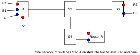
In the diagram above, S1 and S3 each have both red and blue ports. The switch network S1-S4 will deliver traffic only when the source and destination ports are the same color. Red packets can be forwarded to the blue VLAN only by passing through the router R, entering R’s red port and leaving its blue port. R may apply firewall rules to restrict red–blue traffic.

When the source and destination ports are on the same switch, nothing needs to be added to the packet; the switch can keep track of the color of each of its ports. However, switch-to-switch traffic must be additionally tagged to indicate the source. Consider, for example, switch S1 above sending packets to S3 which has nodes R3 (red) and B3 (blue). Traffic between S1 and S3 must be tagged with the color, so that S3 will know to what ports it may be delivered. The IEEE 802.1Q protocol is typically used for this packet-tagging; a 32-bit “color” tag is inserted into the Ethernet header after the source address and before the type field. The first 16 bits of this field is 0x8100, which becomes the new Ethernet type field and which identifies the frame as tagged.

Double-tagging is possible; this would allow an ISP to have one level of tagging and its customers to have another level.

2.7   Epilog

Ethernet dominates the LAN layer, but is not one single LAN protocol: it comes in a variety of speeds and flavors. Higher-speed Ethernet seems to be moving towards fragmenting into a range of physical-layer options for different types of cable, but all based on switches and point-to-point linking; different Ethernet types can be interconnected only with switches. Once Ethernet finally abandons physical links that are bi-directional (half-duplex links), it will be collision-free and thus will no longer need a minimum packet size.

Other wired networks have largely disappeared (or have been renamed “Ethernet”). Wireless networks, however, are here to stay, and for the time being at least have inherited the original Ethernet’s collision-management concerns.

2.8   Exercises

1. Simulate the contention period of five Ethernet stations that all attempt to transmit at T=0 (presumably when some sixth station has finished transmitting). Assume that time is measured in slot times, and that exactly one slot time is needed to detect a collision (so that if two stations transmit at T=1 and collide, and one of them chooses a backoff time k=0, then that station will transmit again at T=2). Use coin flips or some other source of randomness.

2. Suppose we have Ethernet switches S1 through S3 arranged as below. All forwarding tables are initially empty.

S1────────S2────────S3───D
│         │         │
A         B         C

(a). If A sends to B, which switches see this packet?

(b). If B then replies to A, which switches see this packet?

(c). If C then sends to B, which switches see this packet?

(d). If C then sends to D, which switches see this packet?

3. Suppose we have the Ethernet switches S1 through S4 arranged as below. All forwarding tables are empty; each switch uses the learning algorithm of 2.4   Ethernet Switches.

              B
              │
              S4
              │
A───S1────────S2────────S3───C
              │
              D

Now suppose the following packet transmissions take place:

• A sends to B
• B sends to A
• C sends to B
• D sends to A

For each switch, list what source nodes (eg A,B,C,D) it has seen (and thus learned about).

4. In the switched-Ethernet network below, find two packet transmissions so that, when a third transmission A⟶D occurs, the packet is delivered to B (that is, it is forwarded out all ports of S2), but is not similarly delivered to C. All forwarding tables are initially empty, and each switch uses the learning algorithm of 2.4   Ethernet Switches.

              B         C
              │         │
A───S1────────S2────────S3───D

Hint: Destination D must be in S3’s forwarding table, but must not be in S2’s.

5. Given the Ethernet network with learning switches below, with (disjoint) unspecified parts represented by ?, explain why it is impossible for a packet sent from A to B to be forwarded by S1 only to S2, but to be forwarded by S2 out all of S2’s other ports.

    ?         ?
    |         |
A───S1────────S2───B

6. In the diagram of 2.4   Ethernet Switches, suppose node D is connected to S5, and, with the tables as shown below the diagram, D sends to B.

(a). Which switches will see this packet, and thus learn about D?

(b). Which of the switches in part (a) do not already know where B is (and will thus forward the packet out all non-arrival interfaces)?

7. Suppose two Ethernet switches are connected in a loop as follows; S1 and S2 have their interfaces 1 and 2 labeled. These switches do not use the spanning-tree algorithm.

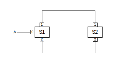
Suppose A attempts to send a packet to destination B, which is unknown. S1 will therefore forward the packet out interfaces 1 and 2. What happens then? How long will A’s packet circulate?

8. The following network is like that of 2.5.1   Example 1: Switches Only, except that the switches are numbered differently. What is the end result of the spanning-tree algorithm in this case?

S1──────S4──────S6
│       │       │
│       │       │
│       │       │
S3──────S5──────S2

9. Suppose you want to develop a new protocol so that Ethernet switches participating in a VLAN all keep track of the VLAN “color” associated with every destination. Assume that each switch knows which of its ports (interfaces) connect to other switches and which may connect to hosts, and in the latter case knows the color assigned to that port.

(a). Suggest a way by which switches might propagate this destination-color information to other switches.

(b). What happens if a port formerly reserved for connection to another switch is now used for a host?