17 Queuing and Scheduling¶

Is giving all control of congestion to the TCP layer really the only option? As the Internet has evolved, so have situations in which we may not want routers handling all traffic on a first-come, first-served basis. Traffic with delay bounds – so-called real-time traffic, often involving either voice or video – is likely to perform much better with preferential service, for example; we will turn to this in 18 Quality of Service. But even without real-time traffic, we might be interested in guaranteeing that each of several customers gets an agreed-upon fraction of bandwidth, regardless of what the other customers are receiving. If we trust only to TCP Reno’s bandwidth-allocation mechanisms, and if one customer has one connection and another has ten, then the bandwidth received may also be in the ratio of 1:10. This may make the first customer quite unhappy.

The fundamental mechanism for achieving these kinds of traffic-management goals in a shared network is through queuing; that is, in deciding how the routers prioritize traffic. In this chapter we will take a look at what router-based strategies are available; in the following chapter we will study how some of these ideas have been applied to develop distributed quality-of-service options.

Previously, in 14.1 A First Look At Queuing, we looked at FIFO queuing – both tail-drop and random-drop variants – and (briefly) at priority queuing. These are examples of queuing disciplines, a catchall term for anything that supports a way to accept and release packets. The RED gateway strategy (14.8.3 RED gateways) could qualify as a separate queuing discipline, too, although one closely tied to FIFO.

Queuing disciplines provide tools for meeting administratively imposed constraints on traffic. Two senders, for example, might be required to share an outbound link equally, or in the proportion 60%-40%, even if one participant would prefer to use 100% of the bandwidth. Alternatively, a sender might be required not to send in bursts of more than 10 packets at a time.

Closely allied to the idea of queuing is scheduling: deciding what packets get sent when. Scheduling may take the form of sending someone else’s packets right now, or it may take the form of delaying packets that are arriving too fast.

While priority queuing is one practical alternative to FIFO queuing, we will also look at so-called fair queuing, in both flat and hierarchical forms. Fair queuing provides a straightforward strategy for dividing bandwidth among multiple senders according to preset percentages.

Also introduced here is the token-bucket mechanism, which can be used for traffic scheduling but also for traffic description.

Some of the material here – in particular that involving fair queuing and the Parekh-Gallager theorem – may give this chapter a more mathematical feel than earlier chapters. Mostly, however, this is confined to the proofs; the claims themselves are more straightforward.

17.1 Queuing and Real-Time Traffic¶

One application for advanced queuing mechanisms is to support real-time transport – that is, traffic with delay constraints on delivery.

In its original conception, the Internet was arguably intended for non-time-critical transport. If you wanted to place a digital phone call where every (or almost every) byte was guaranteed to arrive within 50 ms, your best bet might be to use the (separate) telephone network instead.

And, indeed, having an entirely separate network for real-time transport is definitely a workable solution. It is, however, expensive; there are many economies of scale to having just a single network. There is, therefore, a great deal of interest in figuring out how to get the Internet to support real-time traffic directly.

The central strategy for mixing real-time and bulk traffic is to use queuing disciplines to give the real-time traffic the service it requires. Priority queuing is the simplest mechanism, though the fair-queuing approach below offers perhaps greater flexibility.

We round out the chapter with the Parekh-Gallager theorem, which provides a precise delay bound for real-time traffic that shares a network with bulk traffic. All that is needed is that the real-time traffic satisfies a token-bucket specification and is assigned bandwidth guarantees through fair queuing; the volume of bulk traffic does not matter. This is exactly what is needed for real-time support.

While this chapter contains some rather elegant theory, it is not at all clear how much it is put into practice today, at least for real-time traffic at the ISP level. We will return to this issue in the following chapter, but for now we acknowledge that real-time traffic management using the queuing mechanisms described here has seen limited acceptance in the Internet marketplace.

17.2 Traffic Management¶

Even if none of your traffic has real-time constraints, you still may wish to allocate bandwidth according to administratively determined percentages. For example, you may wish to give each of three departments an equal share of download (or upload) capacity, or you may wish to guarantee them shares of 55%, 35% and 10%. If you want any unused capacity to be divided among the non-idle users, fair queuing is the tool of choice, though in some contexts it may require cooperation from your ISP. If the users are more like customers receiving only the bandwidth they pay for, you might want to enforce flat caps even if some bandwidth thus goes unused; token-bucket filtering would then be the way to go. If bandwidth allocations are not only by department (or customer) but also by workgroup (or customer-specific subcategory), then hierarchical queuing offers the necessary control.

In general, network management divides into managing the hardware and managing the traffic; the tools in this chapter address this latter component. These tools can be used internally by ISPs and at the customer/ISP interconnection, but traffic management often makes good economic sense even when entirely contained within a single organization.

17.3 Priority Queuing¶

To get started, let us fill in the details for priority queuing, which we looked at briefly in 14.1.1 Priority Queuing. Here a given outbound interface can be thought of as having two (or more) physical queues representing different priority levels. Packets are placed into the appropriate subqueue based on some packet attribute, which might be an explicit priority tag, or which might be the packet’s destination socket. Whenever the outbound link becomes free and the router is able to send the next packet, it always looks first to the higher-priority queue; if it is nonempty then a packet is dequeued from there. Only if the higher-priority queue is empty is the lower-priority queue served.

Note that priority queuing is nonpreemptive: if a high-priority packet arrives while a low-priority packet is being sent, the latter is not interrupted. Only when the low-priority packet has finished transmission does the router again check its high-priority subqueue(s).

Priority queuing can lead to complete starvation of low-priority traffic, but only if the high-priority traffic consumes 100% of the outbound bandwidth. Often we are able to guarantee (for example, through admission control) that the high-priority traffic is limited to a designated fraction of the total outbound bandwidth.

17.4 Queuing Disciplines¶

As an abstract data type, a queuing discipline is simply a data structure that supports the following operations:

enqueue()
dequeue()
is_empty()

Note that the enqueue() operation includes within it a way to handle dropping a packet in the event that the queue is full. For FIFO queuing, the enqueue() operation needs only to know the correct outbound interface; for priority queuing enqueue() also needs to be told – or be able to infer – the packet’s priority classification.

We may also in some cases find it convenient to add a peek() operation to return the next packet that would be dequeued if we were actually to do that, or at least to return some important statistic (eg size or arrival time) about that packet.

As with FIFO and priority queuing, any queuing discipline is always tied to a specific outbound interface. In that sense, any queuing discipline has a single output.

On the input side, the situation may be more complex. The FIFO queuing discipline has a single input stream, though it may be fed by multiple physical input interfaces: the enqueue() operation puts all packets in the same physical queue. A queuing discipline may, however, have multiple input streams; we will call these classes, or subqueues, and will refer to the queuing discipline itself as classful. Priority queues, for example, have an input class for each priority level.

When we want to enqueue a packet for a classful queuing discipline, we must first invoke a classifier – possibly external to the queuing discipline itself – to determine the input class. (In the linux documentation, what we have called classifiers are often called filters.) For example, if we wish to use a priority queue to give priority to VoIP packets, the classifier’s job is to determine which arriving packets are in fact VoIP packets (perhaps taking into account things like size or port number or source host), so as to be able to provide this information to the enqueue() operation. The classifier might also take into account pre-existing traffic reservations, so that packets that belong to flows with reservations get preferred service, or else packet tags that have been applied by some upstream router; we return to both of these in 18 Quality of Service.

The number and configuration of classes is often fixed at the time of queuing-discipline creation; this is typically the case for priority queues. Abstractly, however, the classes can also be dynamic; an example of this might be fair queuing (below), which often supports a configuration in which a separate input class is created on the fly for each separate TCP connection.

FIFO and priority queuing are both work-conserving, meaning that the associated outbound interface is not idle unless the queue is empty. A non-work-conserving queuing discipline might, for example, artificially delay some packets in order to enforce an administratively imposed bandwidth cap. Non-work-conserving queuing disciplines are often called traffic shapers or policers; see 17.9 Token Bucket Filters below for an example.

17.5 Fair Queuing¶

An important alternative to FIFO and priority is fair queuing. Where FIFO and its variants have a single input class and put all the incoming traffic into a single physical queue, fair queuing maintains a separate logical FIFO subqueue for each input class; we will refer to these as the per-class subqueues. Division into classes can be fine-grained – eg a separate class for each TCP connection – or coarse-grained – eg a separate class for each arrival interface, or a separate class for each designated internal subnet.

Suppose for a moment that all packets are the same size; this makes fair queuing much easier to visualize. In this (special) case – sometimes called Nagle fair queuing, and proposed in RFC 970 – the router simply services the per-class subqueues in round-robin fashion, sending one packet from each in turn. If a per-class subqueue is empty, it is simply skipped over. If all per-class subqueues are always nonempty this resembles time-division multiplexing. However, unlike time-division multiplexing if one of the per-class subqueues does become empty then it no longer consumes any outbound bandwidth. Recalling that all packets are the same size, the total bandwidth is then divided equally among the nonempty per-class subqueues; if there are K such queues, each will get 1/K of the output.

Fair queuing was extended to streams of variable-sized packets in [DKS89] and [LZ89]. Since then there has been considerable work in trying to figure out how to implement fair queuing efficiently and to support appropriate variants.

17.5.1 Weighted Fair Queuing¶

A straightforward extension of fair queuing is weighted fair queuing (WFQ), where instead of giving each class an equal share, we assign each class a different percentage. For example, we might assign bandwidth percentages of 10%, 30% and 60% to three different departments. If all three subqueues are active, each gets the listed percentage. If the 60% subqueue is idle, then the others get 25% and 75% respectively, preserving the 1:3 ratio of their allocations. If the 10% subqueue is idle, then the other two subqueues get 33.3% and 66.7%.

Weighted fair queuing is, conceptually, a straightforward generalization of fair queuing, although the actual implementation details are sometimes nontrivial as the round-robin implementation above naturally yields equal shares. If all packets are still the same size, and we have two per-class subqueues that are to receive allocations of 40% and 60% (that is, in the ratio 2:3), then we could implement WFQ by having one per-class subqueue send two packets and the other three. Or we might intermingle the two: class 1 sends its first packet, class 2 sends its first packet, class 1 sends its second, class 2 sends its second and its third. If the allocation is to be in the ratio 1:√2, the first sender might always send 1 packet while the second might send in a pattern – an irregular one – that averages √2: 1, 2, 1, 2, 1, 1, 2, ....

The fluid-based GPS model approach to fair queuing, 17.5.4 The GPS Model, does provide an algorithm that has direct, natural support for weighted fair queuing.

17.5.2 Different Packet Sizes¶

If not all the packets are the same size, fair queuing and weighted fair queuing are still possible but we have a little more work to do. This is an important practical case, as fair queuing is often used when one input class consists of small-packet real-time traffic.

We present two mechanisms for handling different-sized packets; the two are ultimately equivalent. The first – 17.5.3 Bit-by-bit Round Robin – is a straightforward extension of the round-robin idea, and the second – 17.5.4 The GPS Model – uses a “fluid” model of simultaneous packet transmission. Both mechanisms share the idea of a “virtual clock” that runs at a rate proportional to the number of active subqueues; as we shall see, the point of varying the clock rate in this way is so that the virtual-clock time at which a given packet would theoretically finish transmission does not depend on activity in any of the other subqueues.

Finally, we present the quantum algorithm – 17.5.5 The Quantum Algorithm – which is a more-efficient approximation to either of the exact algorithms, but which – being an approximation – no longer satisfies a sometimes-important time constraint.

For a straightforward generalization of the round-robin idea to different packet sizes, we start with a simplification: let us assume that each per-class subqueue is always active, where a subqueue is active if it is nonempty whenever the router looks at it.

If each subqueue is always active for the equal-sized-packets case, then packets are transmitted in order of increasing (or at least nondecreasing) cumulative data sent by each subqueue. In other words, every subqueue gets to send its first packet, and only then do we go on to begin transmitting second packets, and so on.

Still assuming each subqueue is always active, we can handle different-sized packets by the same idea. For packet P, let C_P be the cumulative number of bytes that will have been sent by P’s subqueue as of the end of P. Then we simply need to send packets in nondecreasing order of C_P.

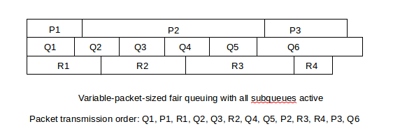
In the diagram above, transmission in nondecreasing order of C_P means transmission in left-to-right order of the vertical lines marking packet divisions, eg Q1, P1, R1, Q2, Q3, R2, .... This ensures that, in the long run, each subqueue gets an equal share of bandwidth.

A completely equivalent strategy, better suited for generalization to the case where not all subqueues are always active, is to send each packet in nondecreasing order of virtual finishing times, calculated for each packet with the assumption that only that packet’s subqueue is active. The virtual finishing time F_P of packet P is equal to C_P divided by the output bandwidth. We use finishing times rather than starting times because if one packet is very large, shorter packets in other subqueues that would finish sooner should be sent first.

17.5.2.1 A first virtual-finish example¶

As an example, suppose there are two subqueues, Q₁ and Q₂. Suppose further that a stream of 1001-byte packets P₁, P₂, P₃, ... arrives at Q₁, and a stream of 400-byte packets R₁, R₂, R₃, ... arrives for Q₂; each stream is steady enough that each subqueue is always active. Finally, assume the output bandwidth is 1 byte per unit time, and let T=0 be the starting point.

For the Q₁ subqueue, the virtual finishing times calculated as above would be P₁ at 1001, P₂ at 2002, P₃ at 3003, etc; for Q₂ the finishing times would be R₁ at 400, R₂ at 800, R₃ at 1200, etc. So the order of transmission of all the packets together will be as follows:

Packet	virtual finish	actual finish
R₁	400	400
R₂	800	800
P₁	1001	1801
R₃	1200	2201
R₄	1600	2601
R₅	2000	3001
P₂	2002	4002

For each packet we have calculated in the table above its virtual finishing time, and then its actual wallclock finishing time assuming packets are transmitted in nondecreasing order of virtual finishing time (as shown).

Because both subqueues are always active, and because the virtual finishing times assumed each subqueue received 100% of the output bandwidth, in the long run the actual finishing times will be about double the virtual times. This, however, is irrelevant; all that matters is the relative virtual finishing times.

The next step is to extend this strategy to the case where subqueues can sometimes be inactive, using the model of bit-by-bit round robin.

17.5.3 Bit-by-bit Round Robin¶

Imagine sending a single bit at a time from each active input subqueue, in round-robin fashion. While not directly implementable, this certainly meets the goal of giving each active subqueue equal service, even if packets are of different sizes. We will use bit-by-bit round robin, or BBRR, as a way of modeling packet-finishing times, and then, as in the previous example, send the packets the usual way – one full packet at a time – in order of increasing BBRR-calculated virtual finishing times.

It will sometimes happen that a larger packet is being transmitted at the point a new, shorter packet arrives for which a smaller finishing time is computed. The current transmission is not interrupted, though; the algorithm is non-preemptive.

The trick to making the BBRR approach workable is to find an “invariant” formulation of finishing time that does not change as later packets arrive, or as other subqueues become active or inactive. To this end, we define the “rounds counter” R(t), where t is the time measured in units of the transmission time for one bit. When there are any active (nonempty or currently transmitting) input subqueues, R(t) counts the number of round-robin cycles that have occurred since the last time all the subqueues were empty. If there are K active input subqueues, then R(t) increments by 1 as t increments by K; that is, R(t) grows at rate 1/K.

An important attribute of R(t) is that, if a packet of size S bits starts transmission via BBRR at R₀ = R(t₀), then it will finish when R(t) = R₀+S, regardless of whether any other input subqueues become active or become empty. For any packet actively being sent via BBRR, R(t) increments by 1 for each bit of that packet sent. If for a given round-robin cycle there are K subqueues active, then K bits will be sent in all, and R(t) will increment by 1.

To calculate the virtual BBRR finishing time of a packet P, we first record R_P = R(t_P) at the moment of arrival. We now compute the BBRR-finishing R-value F_P as follows; we can think of this as a “time” measured via the rounds counter R(t). That is, R(t) represents a “virtual clock” that happens sometimes to run slow. Let S be the size of the packet P in bits. If P arrived on a previously empty input subqueue, then its BBRR transmission can begin immediately, and so its finishing R-value F_P is simply R_P+S. If the packet’s subqueue was nonempty, we look up the (future) finishing R-value of the packet immediately ahead of P in its subqueue, say F_prev; the finishing R-value of P is then F_P = F_prev + S. This is sometimes described as:

Start = max(R(now), F_prev)

F_P = Start + S (S = packet size, measured in bits)

As each new packet P arrives, we calculate its BBRR-finishing R-value F_P, and then send packets the conventional one-packet-at-a-time way in increasing order of F_P. As stated above, F_P will not change if other subqueues empty or become active, thus changing the rate of the rounds-counter R(t).

The router maintaining R(t) does not have to increment it on every bit; it suffices to update it whenever a packet arrives or a subqueue becomes empty. If the previous value of R(t) was R_prev, and from then to now exactly K subqueues were nonempty, and M bit-times have elapsed according to the wall clock, then the current value of R(t) is R_prev + M/K.

17.5.3.1 BBRR example¶

As an example, suppose the fair queuing router has three input subqueues Q₁, Q₂ and Q₃, initially empty. The following packets arrive at the wall-clock times shown.

Packet	Queue	Size	Arrival time, t
P₁₁	Q₁	1000	0
P₁₂	Q₁	1000	0
P₂₁	Q₂	600	800
P₂₂	Q₂	400	800
P₂₃	Q₂	400	800
P₃₁	Q₃	200	1200
P₃₂	Q₃	200	2100

At t=0, we have R(t)=0 and we assign finishing R-values F₁₁=1000 to P₁₁ and F₁₂ = F₁₁+1000 = 2000 to P₁₂. Transmission of P₁₁ begins.

When the three Q₂ packets arrive at t=800, we have R(t)=800 as well, as only one subqueue has been active. We assign finishing R-values for the newly arriving P₂₁, P₂₂ and P₂₃ of F₂₁ = 800+600 = 1400, F₂₂ = 1400+400 = 1800, and F₂₃ = 1800+400 = 2200. At this point, BBRR begins serving two subqueues, so the R(t) rate is cut in half.

At t=1000, transmission of packet P₁₁ is completed; R(t) is 800 + 200/2 = 900. The smallest finishing R-value on the books is F₂₁, at 1400, so P₂₁ is the second packet transmitted. P₂₁‘s real finishing time will be t = 1000+600 = 1600.

At t=1200, P₃₁ arrives; transmission of P₂₁ is still in progress. R(t) is 800 + 400/2 = 1000; we calculate F₃₁ = 1000 + 200 = 1200. Note this is less than the finishing R-value for P₂₁, which is currently transmitting, but P₂₁ is not preempted. At this point (t=1200, R(t)=1000), the R(t) rate falls to 1/3.

At t=1600, P₂₁ has finished transmission. We have R(t) = 1000 + 400/3 = 1133. The next smallest finishing R-value is F₃₁ = 1200 so transmission of P₃₁ commences.

At t=1800, P₃₁ finishes. We have R(1800) = R(1200) + 600/3 = 1000 + 200 = 1200 (3 subqueues have been busy since t=1200). Q₃ is now empty, so the R(t) rate rises from 1/3 to 1/2. The next smallest finishing R-value is F₂₂=1800, so transmission of P₂₂ begins. It will finish at t=2200.

At t=2100, we have R(t) = R(1800) + 300/2 = 1200 + 150 = 1350. P₃₂ arrives on Q₃; it is assigned a finishing time of F₃₂ = 1350 + 200 = 1550. Again, transmission of P₂₂ is not preempted even though F₃₂ < F₂₂. The R(t) rate again falls to 1/3.

At t=2200, P₂₂ finishes. R(t) = 1350 + 100/3 = 1383. The next smallest finishing R-value is F₃₂=1550, so transmission of P₃₂ begins.

At t=2400, transmission of P₃₂ ends. R(t) is now 1350 + 300/3 = 1450. The next smallest finishing R-value is F₁₂ = 2000, so transmission of P₁₂ begins. The R(t) rate rises to 1/2, as Q₃ is again empty.

At t=3400, transmission of P₁₂ ends. R(t) is 1450 + 1000/2 = 1950. The only remaining unsent packet is P₂₃, with F₂₃=2200. We send it.

At t=3800, transmission of P₂₃ ends. R(t) is 1950 + 400/1 = 2350.

To summarize:

Packet	send-time, wall clock t	calculated finish R-value	R-value when sent	R-value at finish
P₁₁	0	1000	0	900
P₂₁	1000	1400	900	1133
P₃₁	1600	1200*	1133	1200
P₂₂	1800	1800	1200	1383
P₃₂	2200	1550*	1383	1450
P₁₂	2400	2000	1450	1950
P₂₃	3400	2200	1950	2350

Packets arrive, begin transmission and finish in “real” time. However, the number of queues active in real time affects the rate of the rounds-counter R(t); this value is then attached to each packet as it arrives as its virtual finishing time, and determines the order of packet transmission.

The change in R-value from start to finish exactly matches the packet size when the packet is “virtually sent” via BBRR. When the packet is sent as an indivisible unit, as in the table above, the change in R-value is usually much smaller, as the R-clock runs slower whenever at least two subqueues are in use.

The calculated-finish R-values are not in fact increasing, as can be seen at the starred (*) values. This is because, for example, P₃₁ was not yet available when it was time to send P₂₁.

Computationally, maintaining the R-value counter is inconsequential. The primary performance issue with BBRR simulation is the need to find the smallest R-value whenever a new packet is to be sent. If n is the number of packets waiting to be sent, then we can do this in time O(log(n)) by keeping the R-values sorted in an appropriate data structure.

The BBRR approach assumes equal weights for each subqueue; this does not generalize completely straightforwardly to weighted fair queuing as the number of subqueues cannot be fractional. If there are two queues, one which is to have weight 40% and the other 60%, we could use BBRR with five subqueues, two of which (2/5) are assigned to the 40%-subqueue and the other three (3/5) to the 60% subqueue. But this becomes increasingly awkward as the fractions become less simple; the GPS model, next, is a better option.

17.5.4 The GPS Model¶

An almost-equivalent model to BBRR is the generalized processor sharing model, or GPS; it was first developed as an application to CPU scheduling. In this approach we imagine the packets as liquid, and the outbound interface as a pipe that has a certain total capacity. The head packets from each subqueue are all squeezed into the pipe simultaneously, each at its designated fractional rate. The GPS model is essentially an “infinitesimal” variant of BBRR. The GPS model has an advantage of generalizing straightforwardly to weighted fair queuing.

Other fluid models have also been used in the analysis of networks, eg for the study of TCP, though we do not consider these here. See [MW00] for one example.

For the GPS model, assume there are N input subqueues, and the ith subqueue, 0≤i<N, is to receive fraction 𝛼_i > 0, where 𝛼₀+𝛼₁+ ... + 𝛼_N−1=1. If at some point a set A of input subqueues is active , say A = {0,2,4}, then subqueue 0 will receive fraction 𝛼₀/(𝛼₀+𝛼₂+𝛼₄), and subqueues 2 and 4 similarly. The router forwards packets from each active subqueue simultaneously, each at its designated rate.

The GPS model (and the BBRR model) provides an ideal degree of isolation between input flows: each flow is insulated from any delay due to packets on competing flows. The ith flow receives bandwidth of at least 𝛼_i and packets wait only for other packets belonging to the same flow. When a packet arrives for an inactive subqueue, forwarding begins immediately, interleaved with any other work the router is doing. Traffic on other flows can reduce the real rate of a flow, but not its virtual rate.

While GPS is convenient as a model, it is even less implementable, literally, than BBRR. As with BBRR, though, we can use the GPS model to determine the order of one-packet-at-a-time transmission. As each real packet arrives, we calculate the time it would finish, if we were using GPS. Packets are then transmitted under WFQ one at a time, in order of increasing GPS finishing time.

In lieu of the BBRR rounds counter R(t), a virtual clock VC(t) is used that runs at an increased rate 1/𝛼 ≥ 1 where 𝛼 is the sum of the 𝛼_i for the active subqueues. That is, if subqueues 0, 2 and 4 are active, then the VC(t) clock runs at a rate of 1/(𝛼₀+𝛼₂+𝛼₄). If all the 𝛼_i are equal, each to 1/N, then VC(t) always runs N times faster than R(t), and so VC(t) = N×R(t); the VC clock runs at wallclock speed when all input subqueues are active and speeds up as subqueues become idle.

For any one active subqueue i, the GPS rate of transmission relative to the virtual clock (that is, in units of bits per virtual-second) is always equal to fraction 𝛼_i of the full output-interface rate. That is, if the output rate is 10 Mbps and an active flow has fraction 𝛼 = 0.4, then it will always transmit at 4 bits per virtual microsecond. When all the subqueues are active, and the VC clock runs at wallclock speed, the flow’s actual rate will be 4 bits/µsec. When the subqueue is active alone, its speed measured by a real clock will be 10 bit/µsec but the virtual clock will run 2.5 times faster so 10 bits/µsec is 10 bits per 2.5 virtual microseconds, or 4 bits per virtual microsecond.

To make this claim more precise, let A be the set of active queues, and let 𝛼 again be the sum of the 𝛼_j for j in A. Then VC(t) runs at rate 1/𝛼 and active subqueue i’s data is sent at rate 𝛼_i/𝛼 relative to wallclock time. Subqueue i’s transmission rate relative to virtual time is thus (𝛼_i/𝛼)/(1/𝛼) = 𝛼_i.

As other subqueues become inactive or become active, the VC(t) rate and the actual transmission rate move in lockstep. Therefore, as with BBRR, a packet P of size S on subqueue i that starts transmission at virtual time T will finish at T + S/(r×𝛼_i) by the VC clock, where r is the actual output rate of the router, regardless of what is happening in the other subqueues. In other words, VC-calculated finishing times are invariant.

To round out the calculation of finishing times, suppose packet P of size S arrives on an active GPS subqueue i. The previous packet in that subqueue will have finishing time F_prev, and that will become P’s start time. If P arrives on an inactive subqueue, GPS allows it to begin transmitting immediately. Either way, as with BBRR, P’s start time is P_start = max(VC(now), F_prev), and its finishing time on the VC clock is F_P = P_start + S/(r×𝛼_i). In one expression, this finishing time is: F_P = max(VC(now), F_prev) + S/(r×𝛼_i)

In 17.8.1.1 WFQ with non-FIFO subqueues below, we will consider WFQ routers that, as part of a hierarchy, are in effect only allowed to transmit intermittently. In such a case, the virtual clock should be suspended whenever output is blocked. This is perhaps easiest to see for the BBRR scheduler: the rounds-counter RR(t) is to increment by 1 for each bit sent by each active subqueue. When no bits may be sent, the clock should not increase.

As an example of what happens if this is not done, suppose R has two subqueues A and B; the first is empty and the second has a long backlog. R normally processes one packet per second. At T=0/VC=0, R’s output is suspended. Packets in the second subqueue b₁, b₂, b₃, ... have virtual finishing times 1, 2, 3, .... At T=10, R resumes transmission, and packet a₁ arrives on the A subqueue. If R’s virtual clock had been suspended for the interval 0≤T≤10, a₁ would be assigned finishing time T=1 and would have priority comparable to b₁. If R’s virtual clock had continued to run, a₁ would be assigned finishing time T=11 and would not be sent until b₁₁ reached the head of the B queue.

17.5.4.1 The WFQ scheduler¶

To schedule actual packet transmission under weighted fair queuing, we calculate upon arrival each packet’s virtual-clock finishing time assuming it were to be sent using GPS. Whenever the sender is ready to start transmission of a new packet, it selects from the available packets the one with the smallest GPS-finishing-time value. By the argument above, a packet’s GPS finishing time does not depend on any later arrivals or idle periods on other subqueues. As with BBRR, small but later-arriving packets might have smaller virtual finishing times, but a packet currently being transmitted will not be interrupted.

17.5.4.2 Finishing Order under GPS and WFQ¶

We now look at the order in which packets finish transmission under GPS versus WFQ. The goal is to provide in 17.5.4.7 Finishing-Order Bound a tight bound on how long packets may have to wait under WFQ compared to GPS. We emphasize again:

GPS finishing time: the theoretical finishing time based on parallel multi-packet transmissions under the GPS model
WFQ finishing time: the real finishing time assuming packets are sent sequentially in increasing order of calculated GPS finishing time

One way to view this is as a quantification of the informal idea that WFQ provides a natural priority for smaller packets, at least smaller packets sent on previously idle subqueues. This is quite separate from the bandwidth guarantee that a given small-packet input class might receive; it means that small packets are likely to leapfrog larger packets waiting in other subqueues. The quantum algorithm, below, provides long-term WFQ bandwidth guarantees but does not provide the same delay assurances.

First, if all subqueues are always active (or if a fixed subset of subqueues is always active), then packets finish under WFQ in the same order as they do under GPS. This is because under WFQ packets are transmitted in the order of GPS finishing times according the virtual clock, and if all subqueues are always active the virtual clock runs at a rate identical to wallclock time (or, if a fixed subset of subqueues is always active, at a rate proportional to wallclock time).

If all subqueues are always active, we can assume that all packets were in their subqueues as of time T=0; the finishing order is the same as long as each packet arrived before its subqueue went inactive.

Finally, if all subqueues are always active then each packet finishes at least as early under WFQ as under GPS. To see this, let P_j be the jth packet to finish, under either GPS or WFQ. At the time when P_j finishes under WFQ, the router R will have devoted 100% of its output bandwidth exclusively to P₁ through P_j. When P_j finishes under GPS, R will also have transmitted P₁ through P_j, and may have transmitted fractions of later packets as well. Therefore, the P_j finishing time under GPS cannot be earlier.

The finishing order and the relative GPS/WFQ finishing times may change, however, if – as will usually be the case – some subqueues are sometimes idle; that is, if packets sometimes “arrive late” for some subqueues.

17.5.4.3 GPS Example 1¶

As a first example we return to the scenario of 17.5.2.1 A first virtual-finish example. The router’s two subqueues are always active; each has an allocation of 𝛼=50%. Packets P₁, P₂, P₃, ..., all of size 1001, wait in the first queue; packets R₁, R₂, R₃, ..., all of size 400, wait in the second queue. Output bandwidth is 1 byte per unit time, and T=0 is the starting point.

The router’s virtual clock runs at wallclock speed, as both subqueues are always active. If F_i represents the virtual finishing time of R_i, then we now calculate F_i as F_i-1 + 400/𝛼 = F_i-1 + 800. The virtual finishing times of P₁, P₂, etc are similarly at multiples of 2002.

Packet	virtual finish	actual finish time
R₁	800	400
R₂	1600	800
P₁	2002	1801
R₃	2400	2201
R₄	3200	2601
R₅	4000	3001
P₂	4004	4002

In the table above, the “virtual finish” column is simply double that of the BBRR version, reflecting the fact that the virtual finishing times are now scaled by a factor of 1/𝛼 = 2. The actual finish times are identical to what we calculated before.

Note that, in every case, the actual WFQ finish time is always less than or equal to the virtual GPS finish time.

17.5.4.4 GPS Example 2¶

If the router has only a single active subqueue, with share 𝛼 and packets P₁, P₂, P₃, ..., then the calculated virtual-clock packet finishing times will be equal to the time on the virtual clock at the point of actual finish, at least if this has been the case since the virtual clock last restarted at T=VC=0. Let r be the output rate of the router, let S₁, S₂, S₃ be the sizes of the packets and let F₁, F₂, F₃ be their virtual finishing times with F₀=0. Then

F_i = F_i-1 + S_i/(r𝛼) = S₁/(r𝛼) + ... + S_i/(r𝛼)

The ith packet’s actual finishing time A_i is (S₁ + ... + S_i)/r, which is 𝛼×F_i. But the virtual clock runs fast by a factor of 1/𝛼, so the actual finishing time on the virtual clock is A_i/𝛼 = F_i.

17.5.4.5 GPS Example 3¶

The next example illustrates a smaller but later-arriving packet, in this case P₄, that finishes ahead of P₃ under GPS but not under WFQ. P₃ can be said to leapfrog P₄ and P₅ under WFQ.

Suppose packets P₁ through P₅ arrive at R at the following times T, and with the following lengths L. The output bandwidth is 1 length unit per time unit; that is, r=1. The total number of length units is 24. Each subqueue is allocated an equal share of the bandwidth; eg 𝛼=1/3.

subqueue 1	subqueue 2	subqueue3
P₁: T=0, L=1	P₂: T=0, L=2	P₅: T=10, L=5
P₃: T=2, L=10	P₄: T=4, L=6

Under WFQ, we send P₁ and then P₂; P₂ is second because its finishing time is later. When P₂ finishes the wallclock time is T=3. At this point, P₃ is the only packet available to send; it finishes at T=13.

Up until T=10, we have two packets in progress under GPS (because P₂ finishes under GPS at T=4 and P₄ arrives at T=4), and so the GPS clock runs at rate 3/2 of wallclock time and the BBRR clock runs at rate 1/2 of wallclock time. At T=4, when P₄ arrives, the BBRR clock is at 2 and the VC clock is at 6 and we calculate the BBRR finishing time as 2+6=8 and the GPS finishing time as 6+6/(1/3) = 24. At T=10, the BBRR clock is at 5 and the GPS clock is 15. P₅ arrives then; we calculate its BBRR finishing time as 5+5=10 and its GPS finishing time as 15+5/𝛼 = 30.

Because P₄ has the earlier virtual-clock finishing time, WFQ sends it next after P₃, followed by P₅.

Here is a diagram of transmission under GPS. The chart itself is scaled to wallclock times. The BBRR clock is on the scale below; the VC clock always runs three times faster.

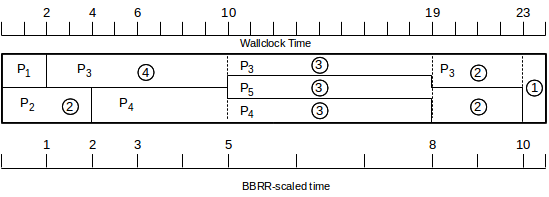
The circled numbers represent the size of the portion of the packet sent in the intervals separated by the dotted vertical lines; for each packet, these add up to the packet’s total size.

Note that, while the transmission order under WFQ is P₁, P₂, P₃, P₄, P₅, the actual finishing order under GPS is P₁, P₂, P₄, P₅, P₃. That is, P₃ managed to leapfrog P₄ and P₅ under WFQ by the simple expedient of being the only packet available for transmission at T=3.

17.5.4.6 GPS Example 4¶

As a second example of leapfrogging, suppose we have the following arrivals; in this scenario, the smaller but later-arriving P₄ finishes ahead of P₁ and P₃ under GPS, but not under WFQ.

subqueue 1	subqueue 2	subqueue3
P₁: T=0, L=1000	P₂: T=0, L=200	P₄: T=600, L=100
	P₃: T=0, L=300

The following diagram shows how the packets shared the link under GPS over time. As can be seen, the GPS finishing order is P₂, P₄, P₃, P₁.

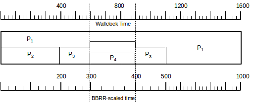
Under WFQ, the transmission order is P₂, P₃, P₁, P₄, because when P₃ finishes at T=500, P₄ has not yet arrived.

17.5.4.7 Finishing-Order Bound¶

These examples bring us to the following delay-bound claim, due to Parekh and Gallager [PG93]; we will make use of it below in 17.13.3 Parekh-Gallager Theorem. It is arguably the deepest part of the Parekh-Gallager theorem.

Claim: For any packet P, the wallclock finishing time of P at a router R under WFQ cannot be later than the wallclock finishing time of P at R under GPS by more than the time R needs to transmit the maximum-sized packet that can appear.

Expressed symbolically, if F_WFQ and F_GPS are the finishing times for P under WFQ and GPS, R’s outbound transmission rate is r, and L_max is the maximum packet size that can appear at R, then

F_WFQ ≤ F_GPS + L_max/r

This is the best possible bound; L_max/r is the time packet P must wait if it has arrived an instant too late and another packet of size L_max has started instead.

Note that, if a packet’s subqueue is inactive, the packet starts transmitting immediately upon arrival under GPS; however, GPS may send the packet relatively slowly.

To prove this claim, let us number the packets P₁ through P_k in order of WFQ transmission, starting from the most recent point when at least one subqueue of the router became active. For each i, let F_i be the finishing time of P_i under WFQ, let G_i be the finishing time of P_i under GPS, and let L_i be the length of P_i; note that, for each i, F_i+1 = L_i+1/r + F_i.

If P_k finishes after P₁ through P_k-1 under GPS, then the argument above (17.5.4.2 Finishing Order under GPS and WFQ) for the all-subqueues-active case still applies to show P_k cannot finish earlier under GPS than it does under WFQ; that is, we have F_k ≤ G_k.

Otherwise, some packet P_i with i<k must finish after P_k under GPS; P_i has leapfrogged P_k under WFQ, presumably because P_k was late in arriving. Let P_m be the most recent (largest m<k) such leapfrogger packet, so that P_m finishes after P_k under GPS but P_m+1 through P_k-1 finish earlier (or are tied); this was illustrated above in 17.5.4.5 GPS Example 3 for k=5 and m=3.

We next claim that none of the packets P_m+1 through P_k could have yet arrived at R at the time T_start when P_m began transmission under WFQ. If some P_i with i>m were present at time T_start, then the fact that it is transmitted after P_m under WFQ would imply that the calculated GPS finishing time came after that of P_m. But, as we argued earlier, calculated virtual-clock GPS finishing times are always the actual virtual-clock GPS finishing times, and we cannot have P_i finishing both ahead of P_m and behind it.

Recalling that F_m is the finishing time of P_m under WFQ, the time T_start above is simply F_m - L_m/r. Between T_start and G_k, all the packets P_m+1 through P_k must arrive and then, under GPS, depart. The absolute minimum time to send these packets under GPS is the WFQ time for end-to-end transmission, which is (L_m+1 + .. + L_k)/r = F_k - F_m. Therefore we have

G_k - T_start ≥ F_k - F_m

G_k - (F_m - L_m/r) ≥ F_k - F_m

F_k ≤ G_k + L_m/r ≤ G_k + L_max/r

The last line represents the desired conclusion.

17.5.5 The Quantum Algorithm¶

The BBRR approach has cost O(log n), where n is the number of packets waiting, as outlined earlier. One simple though approximate alternative that has O(1) performance, introduced in [SV96], is to give each input queue a quantum. At each round, a queue will be able to send a quantum’s worth of packets (plus, as we shall see, a carryover from the previous round). The quantum must be a number of bytes at least as large as the network MTU (so each time a per-class queue has a chance to send, it will be able to send at least one packet). Then, we again service the queues in round-robin fashion, but each time we take as many packets from the queue as we can such that the total size does not exceed the quantum.

One cost of the quantum approach is that the elegant delay bound of 17.5.4.7 Finishing-Order Bound no longer holds. In fact, a sender may be forced to wait for all other senders each to send a full quantum, even if the sender has only a small packet.

If we just allow senders to send up to a quantum’s worth of bytes, the strategy will be biased against classes that, for example, only include packets with size just over half the quantum. Fairness can be improved significantly by keeping track of the difference between the quantum and what was actually sent; we will call this the deficit. If the quantum is 1000 bytes and we have two 600-byte packets, the first of the packets is sent and the deficit is recorded as 400; if we have two 400-byte packets then the deficit is 0 as sending the two 400-byte packets empties the queue.

The next time that queue is serviced, we add the previous deficit to the quantum, and send packets up to a total cumulative size of deficit+quantum. With this variation, if the quantum is 1000 bytes and a steady stream of 600-byte packets arrives on one subqueue, they are sent as follows

round	quantum + prev deficit	packets sent	new deficit
1	1000	1	400
2	1400	2,3	200
3	1200	4,5	0

In three rounds the queue has been allowed to send 5×600 = 3000 bytes, which is exactly 3 quantums. We will refer to this strategy, with provision for deficits as above, as the quantum algorithm for fair queuing. If an input queue is ever empty, its deficit should immediately expire.

We can implement weighted fair queuing using the quantum algorithm by adjusting the quantum sizes in proportion to the weights; that is, if the weights are 40% and 60% then the respective quanta might be 1000 bytes and 1500 bytes. The quantum should be at least as large as the largest packet (eg the MTU), so that if one input class is to have 10% weight and the other 90%, then the second class will have a quantum of 9 times the MTU. Of course, if the smaller-weighted class happens to be a VoIP stream with smaller packets as well, this is less of an issue.

17.5.6 Stochastic Fair Queuing¶

Stochastic fair queuing [McK90] is a different kind of approximation to fair queuing. The ideal is to give each individual TCP connection through a router its own fair queuing class, so that no connection has an incentive to keep more than the minimum number of packets in the queue. However, managing so many separate (and dynamically changing) input classes is computationally intensive. Instead, a hash function is used to put each TCP connection (as identified by its socketpair) into one of several buckets (the current default bucket count is 1024). The buckets are then used as the fair queuing input queues.

If two connections hash to the same bucket, each will get only half the bandwidth to which it is entitled. Therefore the hash function has some additional parameters that allow it to be perturbed at regular intervals; after perturbation, socketpairs that formerly hashed to the same bucket likely now will not.

Stochastic fair queuing is available in the linux kernel.

17.6 Applications of Fair Queuing¶

As we saw in the Queue-Competition Rule in 14.2.2 Example 2: router competition, if a bottleneck router uses FIFO queuing then it pays a sender, in terms of the bandwidth it receives, to keep as many packets as possible in the queue. Fair queuing, however, can behave quite differently. If fair queuing is used with a separate class for each connection, this “greediness” benefit evaporates; a sender need only keep its per-class queue nonempty in order to be guaranteed its assigned share. Senders can limit their queue utilization to one or two packets without danger of being crowded out by competing traffic.

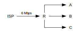
As another application of fair queuing, suppose we have three web servers, A, B and C, to which we want to give equal shares at sending along a 6 Mbps link; all three reach the link through router R. One way would be to have R restrict them each to 2 Mbps, but that is not work-conserving: if one server is idle then its share goes unused. Fair queuing offers a better approach: if all three are busy, each gets 2 Mbps; if two are busy then each gets 3 Mbps, and if only one is busy it gets 6 Mbps. ISPs can also use this strategy internally whenever they have several flows competing for one outbound link.

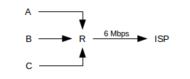
Unfortunately, this strategy does not work quite as well with three receivers. Suppose now A, B and C are three pools of users (eg three departments), and we want to give them each equal shares of an inbound 6 Mbps link:

Inbound fair queuing could be used at the ISP (upstream) end of the connection, where the three flows would be identified by their destinations. But the ISP router is likely not ours to play with. Once the three flows arrive at R, it is too late to allocate shares; there is nothing to do but deliver the traffic to A, B and C respectively. We will return to this scenario below in 17.10 Applications of Token Bucket.

Note that for these kinds of applications we need to be able to designate administratively how packets get classified into different input classes. The automatic classification of stochastic fair queuing, above, will not help here.

17.7 Hierarchical Queuing¶

Any queuing discipline with multiple input classes can participate in a hierarchy: the root queuing discipline is at the top of the tree, and each of its input classes is fed by a separate lower-level queuing discipline.

The usual understanding of hierarchical queuing is that the non-leaf queuing-discipline nodes are “virtual”: they do not store data, but only make decisions as to which subqueue to serve. The only physical output interface is at the root, and all physical queues are attached to the leaf nodes. Each non-leaf queuing-discipline node is allowed to peek at what packet, if any, its subqueues would dequeue if asked, but any node will only actually dequeue a packet unless that packet will immediately be forwarded up the tree to the root. This might be referred to as a leaf-storage hierarchy.

An immediate corollary is that leaf nodes, which now hold all the physical packets, will do all the packet dropping.

While it is possible to chain real queue objects together with real links, to construct composite queuing structures in which packets are not stored only at leaf nodes, the resultant internal-storage hierarchy will often not function as might be expected. For example, a priority-queuing node that immediately forwards each arriving packet on to its parent has forfeited any control over the priority order of resultant packet transmissions. Similarly, if we try to avoid the complexity of hierarchical fair queuing, below, by connecting separate WFQ nodes into a tree with real links, then either packets simply pile up at the root, or else the interior links become the bottleneck. For a case where the internal-storage construction does work, see the end of 17.12 Hierarchical Token Bucket.

17.7.1 Generic Hierarchical Queuing¶

One simple way to enable lazy dequeuing is to require the following properties of the hierarchy’s component queuing disciplines:

each node supports a peek() operation to return the packet it would dequeue if asked, and
any non-leaf node can determine what packet it would itself dequeue simply by calling peek() on each of its child nodes

With these in place, a dequeue operation at the root node will trigger a depth-first traversal of the entire tree through peek() calls; eventually one leaf node will dequeue its packet and pass it up towards the root. We will call this generic hierarchical queuing.

Note that if we have a peek() operation at the leaf nodes, and the second property above for the interior nodes, we can recursively define peek() at every node.

Many homogeneous queuing-discipline hierarchies support this generic mechanism. Priority queuing, as in the example below, works, because when a parent node needs to dequeue a packet it finds the highest-priority nonempty child subqueue, dequeues a packet from it, and sends it up the tree. In this case we do not even need peek(); all we need is is_empty(). Homogeneous FIFO queuing also works, assuming packets are each tagged with their arrival time, because for a node to determine which packet it would dequeue it needs only to peek() at its child nodes and find the earliest-arriving packet.

As an example of where generic hierarchical queuing does not work, imagine a hierarchy consisting of a queuing discipline node that sends the smallest packet first, fed by two FIFO child nodes. The parent would have to dequeue all packets from the child nodes to determine the smallest.

Fair queuing is not quite well-behaved with respect to generic hierarchical queuing. There is no problem if all packets are the same size; in this case the nodes can all implement simple round-robin selection in which they dequeue a packet from the next nonempty child node and send it immediately up the tree. Suppose, however, that to accommodate packets of different sizes all nodes use BBRR (or GPS). The problem is that without timely notification of when packets arrive at the leaf nodes, the interior nodes may not have enough information to determine the correct rates for their virtual clocks. An appropriate fair-queuing-specific modification to the generic hierarchical-queuing algorithm is below in 17.8.1 A Hierarchical Weighted Fair Queuing Algorithm.

17.7.2 Hierarchical Examples¶

Our first example is of hierarchical priority queuing, though as we shall see shortly it turns out in this case that the hierarchy collapses. It may still serve to illustrate some principles, however. The basic queuing-discipline unit will be the two-input-class priority queue, with priorities 0 (high) and 1 (low). We put one of these at the root, named QR, and then put a pair of such queues (QA and QB in the diagram) at the next level down, each feeding into one of the input classes of the root queue.

We now need a classifier: something that can place input packets into one of the four leaf nodes labeled A, B, C and D above; these likely represent FIFO queues. Once everything is set up, the dequeuing rules are as follows:

at the root node, we first see if packets are available in the left (high-priority) subqueue, QA. If so, we dequeue the packet from there; if not, we go on to the right subqueue QB.
at either QA or QB, we first see if packets are available in the left input, labeled 0; if so, we dequeue from there. Otherwise we see if packets are available from the right input, labeled 1. If neither, then the subqueue is empty.

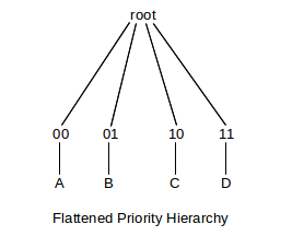
The catch here is that hierarchical priority queuing collapses to a single layer, with four priority levels 00, 01, 10, and 11 (from high to low):

For many other queuing disciplines, however, the hierarchy does not collapse. One example of this might be a root queuing discipline PQR using priority queuing, with two leaf nodes using fair queuing, FQA and FQB. (Fair queuing does not behave well as an interior node without modification, as mentioned above, but it can participate in generic hierarchical queuing just fine as a leaf node.)

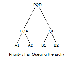
Senders A1 and A2 receive all the bandwidth, if either is active; when this is the case, B1 and B2 get nothing. If both A1 and A2 are active, they get equal shares. Only when neither is active do B1 and B2 receive anything, in which case they divide the bandwidth fairly between themselves. The root node will check on each dequeue() operation whether FQA is nonempty; if it is, it dequeues a packet from FQA and otherwise dequeues from FQB. Because the root does not dequeue a packet from FQA or FQB unless it is about to return it via its own dequeue() operation, those two child nodes do not have to decide which of their internal per-class queues to service until a packet is actually needed.

17.8 Hierarchical Weighted Fair Queuing¶

Hierarchical weighted fair queuing is an elegant mechanism for addressing naturally hierarchical bandwidth-allocation problems, even if it cannot be properly implemented by “generic” methods of creating queuing-discipline hierarchies. There are, fortunately, algorithms specific to hierarchical fair queuing.

The fluid model provides a convenient reference point for determining the goal of hierarchical weighted fair queuing. Each interior node divides its bandwidth according to the usual one-level WFQ mechanism: if N is an interior node, and if the ith child of N is guaranteed fraction 𝛼_i of N’s bandwidth, and A is the set of N’s currently active children, then WFQ on N will allocate to active child j the fraction 𝛽_j equal to 𝛼_j divided by the sum of the 𝛼_i for i in A.

Now we can determine the bandwidth allocated to each leaf node L. Suppose L is at level r (with the root at level 0), and let 𝛽_k be the fraction currently assigned to the node on the root-to-L path at level 0<k≤r. Then L should receive service in proportion to 𝛽₁×...×𝛽_r, the product of the fractions along the root-to-L path. For example, in the following hierarchical model, leaf node L1 should receive fraction 70%×40%×50% = 14% of the total bandwidth.

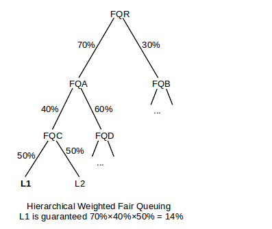
If, however, node FQD becomes inactive, then FQA will assign 100% to FQC, in which case L1 will receive 70%×100%×50% = 35% of the bandwidth.

Alternatively, we can stick to real packets, but simplify by assuming all are the same size and that child allocations are all equal; in this situation we can implement hierarchical fair queuing via generic hierarchical queuing. Each parent node simply dequeues from its child nodes in round-robin fashion, skipping over any empty children.

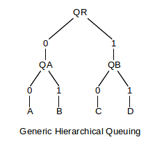
Hierarchical fair queuing – unlike priority queuing – does not collapse; the hierarchical queuing discipline is not equivalent to any one-level queuing discipline. Here is an example illustrating this. We form a tree of three fair queuing nodes, labeled FQR, FQA and FQB in the diagram. Each grants 50% of the bandwidth to each of its two input classes.

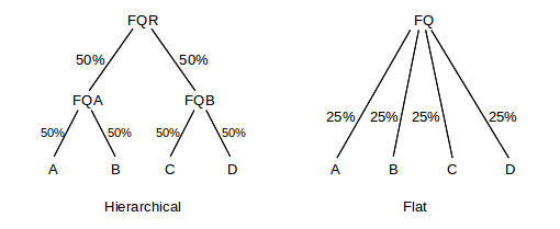
If all four input classes A,B,C,D are active in the hierarchical structure, then each gets 25% of the total bandwidth, just as for a flat four-input-class fair queuing structure. However, consider what happens when only A, B and C are active, and D is idle. In the flat model, A, B and C each get 33%. In the hierarchical model, however, as long as FQA and FQB are both active then each gets 50%, meaning that A and B split FQA’s allocation and receive 25% each, while C gets 50%.

As an application, suppose two teams, Left and Right, are splitting a shared outbound interface; each team has contracted to receive at least 50% of the bandwidth. Each team then further subdivides its allocation among its own members, again using fair queuing. When A, B and C are the active senders, then Team Right – having active sender C – still expects to receive its contractual 50%. Team Right may in fact have decided to silence D specifically so C would receive the full allocation.

Hierarchical fair queuing can not be implemented by computing a finishing time for each packet at the point it arrives. By way of demonstration, consider the following example from [BZ97], with root node R and interior child node C.

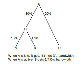
If A is idle, but B and D are active, then B should receive four times the bandwidth of D. Assume for a moment that a large number of packets have arrived for each of B and D. Then B should receive the entire 80% of C’s share. If transmission order can be determined by packet arrival, then the order will look something like

d₁, b₁, b₂, b₃, b₄,

d₂, b₅, b₆, b₇, b₈, ...

Now suppose A wakes up and becomes active. At that point, B goes from receiving 80% of the total bandwidth to 5% = 80% × 1/16, or from four times D’s bandwidth to a quarter of it. The new b/d relative rate, not showing A’s packets, must be

b₁, d₁, d₂, d₃, d₄,

b₂, d₅, d₆, d₇, d₈, ...

The relative frequencies of B and D packets have been reversed by the arrival of later A packets. The packet order for B and D is thus dependent on later arrivals on another queue entirely, and thus cannot be determined at the point the packets arrive.

After presenting the actual hierarchical-WFQ virtual-clock algorithm, we will return to this example in 17.8.1.2 A Hierarchical-WFQ Example.

17.8.1 A Hierarchical Weighted Fair Queuing Algorithm¶

The GPS-based WFQ scheduling algorithm is almost suitable for use in the generic-hierarchical-queuing framework; two adjustments must be made. The first adjustment is that each non-leaf node must be notified whenever any of its formerly empty subqueues becomes active; the second adjustment is a modification to how – and more importantly when – a packet’s virtual finishing time is calculated.

As for the active-subqueue notification, each non-leaf node can, of course, check after dequeuing each packet which of its subqueues is active, using the is_empty() operation. This, however, may be significantly after the subqueue-activating packet has arrived. A WFQ node needs to know the exact time when a subqueue becomes active both to record the GPS virtual-clock start time for the subqueue, and to know when to change the rate of its virtual clock.

Addition of this subqueue-activation notification to hierarchical queuing is straightforward. When a previously empty leaf node receives a packet, it must send a notification to its parent. Each interior node of the hierarchy must in turn forward any received subqueue-activation notification to its parent, provided that none of its other child subqueues were already active. If the interior node already had other active subqueues, then that node is itself active and no new notification needs to be sent. In this way, when a leaf node becomes active, the news will be propagated towards the root of the tree until either the root or an already-active interior node is reached.

To complete the hierarchical WFQ algorithm, we next describe how to modify the algorithm of 17.5.4 The GPS Model to support subqueues of any type (eg FIFO, priority, or in our case hierarchical subtrees), provided inactive subqueues notify the WFQ parent when they become active.

17.8.1.1 WFQ with non-FIFO subqueues¶

Suppose we want to implement WFQ where the per-class subqueues, instead of being FIFO, can be arbitrary queuing disciplines; again, the case in which we are interested is when the subqueue represents a sub-hierarchy. The order of dequeuing from each subqueue might be changed by later arrivals (eg as in priority queuing), and packets in the subqueues might even disappear (as with random-drop queuing). (We will assume that nonempty subqueues can only become empty through a dequeuing operation; this holds in all the cases we will consider here.) The original WFQ algorithm envisioned labeling each packet P with its finishing time as follows:

F_P = max(VC(now), F_prev) + S/𝛼_i

Clearly, this labeling of each packet upon its arrival is incompatible with subqueues that might place later-arriving packets ahead of earlier-arriving ones. The original algorithm must be modified.

It turns out, though, that a WFQ node need only calculate finishing times F_P for the packets P that are at the heads of each of its subqueues, and even that needs only to be done at the time the dequeue() operation is invoked. No waiting packet needs to be labeled. In fact, a packet P1 might be at the head of one subqueue, and be passed over in a dequeue() operation for too large an F_P1, only to be replaced by a different packet P2 during the next dequeue() call.

It is sufficient for the WFQ node to maintain, for each of its subqueues, a variable NextStart, representing the virtual-clock time (according to the WFQ node’s own virtual clock) to be used as the start time for that subqueue’s next transmitted packet. A subqueue’s NextStart value serves as the max(VC(now), F_prev) of the single-layer WFQ formula above. When the parent WFQ node is called upon to dequeue a packet, it calls the peek() operation on each of its subqueues and then calculates the finishing time F_P for the packet P currently at the head of each subqueue as NextStart + size(P)/𝛼, where 𝛼 is the bandwidth fraction assigned to the subqueue.

If a formerly inactive subqueue becomes active, it by hypothesis notifies the parent WFQ node. The parent node records the time on its virtual clock as the NextStart value for that subqueue. Whenever a subqueue is called upon to dequeue packet P, its NextStart value is updated to NextStart + size(P)/𝛼, the virtual-clock finishing time for P.

The active-subqueue notification is also exactly what is necessary for the WFQ node to maintain its virtual clock. If A is the set of active subqueues, and the ith subqueue has bandwidth share 𝛼_i, then the clock is to run at rate equal to the reciprocal of the sum of the 𝛼_i for i in A. This rate needs to be updated whenever a subqueue becomes active or inactive. In the first case, the parent node is notified by hypothesis, and the second case happens only after a dequeue() operation.

There is one more modification needed for non-root WFQ nodes: we must suspend their virtual clocks when they are not “transmitting”, following the argument at the end of 17.5.4 The GPS Model. Non-root nodes do not have real interfaces and do not physically transmit. However, we can say that an interior node N is logically transmitting when the root node R is currently transmitting a packet from leaf node L, and N lies on the path from R to L. Note that all interior nodes on the path from R to L will be logically transmitting simultaneously. For a specific non-root node N, whenever it is called upon at time T to dequeue a packet P, its virtual clock should run during the wallclock interval from T to T + size(P)/r, where r is the root node’s physical bandwidth. The virtual finishing time of P need not have any direct correspondence to this actual finishing time T + size(P)/r. The rate of N’s virtual clock in the interval from T to T + size(P)/r will depend, of course, on the number of N’s active child nodes.

We remark that the dequeue() operation described above is relatively inefficient; each dequeue() operation by the root results in recursive traversal of the entire tree. There have been several attempts to improve the algorithm performance. Other algorithms have also been used; the mechanism here has been taken from [BZ97].

17.8.1.2 A Hierarchical-WFQ Example¶

Let us consider again the example at the end of 17.8 Hierarchical Weighted Fair Queuing:

Assume that all packets are of size 1 and R transmits at rate 1 packet per second. Initially, suppose FIFO leaf nodes B and D have long backlogs (eg b₁, b₂, b₃, ...) but A is idle. Both of R’s subqueues are active, so R’s virtual clock runs at the wall-clock rate. C’s virtual clock is running 16× fast, though. R’s NextStart values for both its subqueues are 0.

The finishing time assigned by R to d_i will be 5i. Whenever packet d_i reaches the head of the D queue, R’s NextStart for D will be 5(i-1). (Although we claimed in the previous section that hierarchical WFQ nodes shouldn’t need to assign finishing times beyond that for the current head packet, for FIFO subqueues this is safe.)

At least during the initial A-idle period, whenever R checks C’s subqueue, if b_i is the head packet then R’s NextStart for C will be 1.25(i-1) and the calculated virtual finishing time will be 1.25i. If ties are decided in B’s favor then in the first ten seconds R will send

b₁, b₂, b₃, b₄, d₁, b₅, b₆, b₇, b₈, d₂

During the ten seconds needed to send the ten packets above, all of the packets dequeued by C come from B. Having only one active subqueue puts C is in the situation of 17.5.4.4 GPS Example 2, and so its packets’ calculated finishing times will exactly match C’s virtual-clock value at the point of actual finish. C dequeues eight packets, so its virtual clock runs for only those 8 of the 10 seconds during which one of the b_i is being transmitted. As a result, packet b_i finishes at time 16i by C’s virtual clock. At T=10, C’s virtual clock is 8×16 = 128.

Now, at T=10, as the last of the ten packets above completes transmission, let subqueue A become backlogged with a₁, a₂, a₃, etc. C will assign a finishing time of 128 + 1.0667i to a_i (1.0667 = 16/15); C has already assigned a virtual finishing time of 9×16=144 to b₉. None of the virtual finishing times assigned by C to the remaining b_i will change.

At this point the virtual finishing times for C’s packets are as follows:

packet	C finishing time	R finishing time
a₁	128 + 1.0667	10 + 1.25
a₂	128 + 2×1.0667	10 + 2.50
a₃	128 + 3×1.0667	10 + 3.75
a₄	128 + 4×1.0667	10 + 5
...
a₁₅	128 + 15×1.0667 = 144	10 + 15×1.25
b₉	144	10 + 16×1.25 = 30

During the time the 16 packets in the table above are sent from C, R will also send four of D’s packets, for a total of 20.

The virtual finishing times assigned by C to b₉ and b₁₀ have not changed, but note that the virtual finishing times assigned to these packets by R are now very different from what they would have been had A remained idle. With A idle, these finishing times would have been F₉ = 11.25 and F₁₀ = 12.50, etc. Now, with A active, it is a₁ and a₂ that finish at 11.25 and 12.50; b₉ will now be assigned by R a finishing time of 30 and b₁₀ will be assigned a finishing time of 50. R is still assigning successive finishing times at increments of 1.25 to packets dequeued by C, but B’s contributions to this stream of packets have been bumped far back.

R’s assignments of virtual finishing times to the d_i are immutable, as are C’s assignments of virtual finishing times, but R can not assign a final virtual finishing time to any of C’s packets (that is, A’s or B’s) until the packet has reached the head of C’s queue. R assigns finishing times to C’s packets in the order they are dequeued, and until a packet is dequeued by C it is subject to potential preemption.

17.9 Token Bucket Filters¶

Token-bucket filters provide an alternative to fair queuing for providing a traffic allocation to each of several groups. The main practical difference between fair queuing and token bucket is that if one sender is idle, fair queuing distributes that sender’s bandwidth among the other senders. Token bucket does not: the bandwidth a sender is allocated is a bandwidth cap.

Suppose the outbound bandwidth is 4 packets/ms and we want to allocate to one particular sender, A, a bandwidth of 1 packet/ms. We could use fair queuing and give sender A a bandwidth fraction of 25%, but suppose we do not want A ever to get more bandwidth than 1 packet/ms. We might do this, for example, because A is paying a reduced rate, and any excess available bandwidth is to be divided among the other senders.

The catch is that we want the flexibility to allow A’s packets to arrive at irregular intervals. We could simply wait 1 ms after each of A’s packets begins transmission, before the next can begin, but this may be too strict. Suppose A has been dutifully submitting packets at 1ms intervals and then the packet that was supposed to arrive at T=6ms instead arrives at T=6.5. If the following packet then arrives on time at T=7, does this mean it should now be held until T=7.5, etc? Or do we allow A to send one late packet at T=6.5 and the next at T=7, on the theory that the average rate is still 1 packet/ms?

The latter option is generally what we want, and the solution is to define A’s quota in terms of a token-bucket specification, which allows for specification of both an average rate and also a burst capacity.

If a packet does not meet the token-bucket specification, it is non-compliant; we can do any of the following things:

delay the packet until the bucket is ready
drop the packet
mark the packet as non-compliant

The first option here is often called shaping; the second, more authoritarian option is sometimes known as policing.

Another use for token-bucket specifications is as a theoretical traffic description, rather than a rule to be enforced; in this context compliance is a non-issue.

A token-bucket filter can be thought of as a queuing discipline, with an underlying FIFO queue. If non-compliant packets are delayed, it is non-work-conserving. Dropping non-compliant packets can be viewed as an alternative to tail-drop. The queuing-discipline definition above in 17.4 Queuing Disciplines does not provide for marking packets, but this is a straightforward extension.

17.9.1 Token Bucket Definition¶

The idea behind a token bucket is that there is a notional bucket somewhere, being filled at a steady rate with tokens (or, if more divisibility is needed, with fluid); any overflow from the bucket is discarded. To send a packet, we need to be able to take one token from the bucket; if the bucket is empty then the packet is non-compliant and must suffer special treatment as above. If the bucket is full, however, then the sender may send a burst of packets corresponding to the bucket capacity (at which point the bucket will be empty).

A common variation is requiring one token per byte rather than per packet, with the fill rate correspondingly scaled; this allows packet size to be taken into account.

More precisely, a token-bucket specification TB(r,B_max) includes a token fill rate of r tokens/sec, representing the rate at which the bucket fills with tokens, and also a bucket capacity (or depth) B_max>0. The bucket fills at the rate specified, subject to a maximum of B_max; we will denote the current capacity by B, or by B(t) if we need to specify the time. In order for a packet of size S (possibly S=1 for counting size in units of whole packets) to be within the specification, the bucket must have at least S tokens; that is, B≥S. Otherwise the packet is non-compliant. When the packet is sent, S tokens are removed from the bucket, that is, B=B−S. It is possible for the packets of a given flow all to be compliant with a given token-bucket specification at one point (eg one router) in the network but not at another point; this can happen, for example, if more than B_max packets pile up at a downstream router due to momentary congestion.

The following graph is a visual representation of a token-bucket constraint. The black and purple curves plotted are of cumulative bits sent as a function of time, that is, bits(t). When bits(t) is horizontal, the sender is idle.

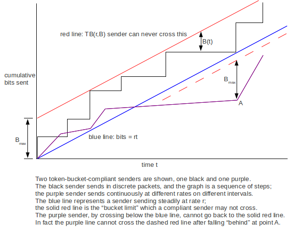
The blue line represents a sender sending linearly at the rate r, with no burstiness. At vertical distance B_max above the blue line is the red line. Graphs for compliant senders cannot cross this, because that would entail a burst of more than B_max above the blue line; we give a more formal argument below. As a sender’s graph approaches the red line, the sender’s current bucket contents decreases; the instantaneous bucket contents for the black sender is shown at one point as B(t).

The purple sender has fallen below the blue line at one point; as a result, it can never catch up. In fact, after passing through the vertex at point A the purple graph can never cross the dashed red line. A proof is in 17.11 Token Bucket Queue Utilization, following some numeric token-bucket examples that illustrate how a token-bucket filter works.

If a packet arrives when there are not enough tokens in the bucket to send it, then as indicated above there are three options. The sender can engage in shaping, making the packet wait until sufficient tokens accumulate. The sender can engage in policing, dropping the packet. Or the sender can send the packet immediately but mark it as noncompliant.

One common strategy is to send noncompliant packets – as marked in the third option above – with lower priority. Alternatively, marked packets may face a greater chance of being dropped by some downstream router. In ATM networks (3.8 Asynchronous Transfer Mode: ATM) the cell-loss priority bit is often used to mark noncompliant packets.

Token-bucket specifications supply a framework for making decisions about admission control: a router can decide whether to accept a new connection (or whether to accept the connection’s quality-of-service request) based on the requested rate and bucket (queue) requirements.

Token-bucket specifications are the mirror-image equivalent to leaky-bucket specifications, in which the fluid leaks out of the leaky bucket at rate r and to send a packet we must add S units without overflowing. The two forms are completely equivalent.

So far we have been using token-bucket specifications to describe traffic; eg traffic arriving at a router. It is also possible to use token buckets to describe the router itself; in this setting, the leaky-bucket formulation may be clearer. The router’s queue represents the bucket, and the router’s packet transmissions represent tokens leaking out of the bucket. Arriving packets are added to the bucket; a bucket overflow represents lost packets. We will not pursue this interpretation further.

17.9.2 Token-Bucket Examples¶

Suppose the token-bucket specification is TB(1/3 packet/ms, 4 packets), and packets arrive at the following times, with the bucket initially full:

0, 0, 0, 2, 3, 6, 9, 12

After all the T=0 packets are processed, the bucket holds 1 token. By the time the fourth packet arrives at T=2, the bucket volume has risen to 1 2/3; it immediately drops to 2/3 when packet 4 is sent. By T=3, the bucket volume has reached 1 and the fifth packet can be sent. The bucket is now empty, but fortunately the remaining packets arrive at 3-ms intervals and can all be sent.

In the next set of packet arrival times, again with TB(1/3,4), we have three bursts of four packets each.

0, 0, 0, 0, 12, 12, 12, 12, 24, 24, 24, 24

Each burst empties the bucket, which then takes 12 ms to refill. All packets are compliant.

In the following set of packet arrival times, still with TB(1/3,4), the burst of four packets at T=0 drains the bucket. At T=3 the bucket size has increased back to 1, allowing the packet that arrives then to be sent but also draining the bucket again.

0, 0, 0, 0, 3, 6, 12, 12

At T=6 the same thing happens. From T=6 to T=12 the bucket contents rise from 0 to 2, allowing the two packets arriving at T=12 to be sent.

Finally, suppose packets arrive at the following times at our TB(1/3,4) filter.

0, 1, 2, 3, 4, 5

Just after T=0 the bucket size is 3; just before T=1 it is 3 1/3.
Just after T=1 the bucket size is 2 1/3; just before T=2 it is 2 2/3
Just after T=2 the bucket size is 1 2/3; just before T=3 it is 2
Just after T=3 the bucket size is 1; just before T=4 it is 1 1/3
Just after T=4 the bucket size is 1/3; just before T=5 it is 2/3
At T=5 the bucket size is 2/3 and the arriving packet is noncompliant.

We can also represent this in tabular form as follows; note that for the noncompliant packet the bucket is not decremented.

packet arrival	0	1	2	3	4	5
bucket just before	4	3 1/3	2 2/3	2	1 1/3	2/3
bucket just after	3	2 1/3	1 2/3	1	1/3	2/3

17.9.3 Multiple Token Buckets¶

It often makes sense to require that a sender comply with two (or more) separate token-bucket specifications. We can think of these being applied to the traffic sequentially. Often one filter will specify a peak rate, with a small bucket size, and the other will specify an average rate, with a larger bucket size. Consider, for example, the following pair:

TB(1 packet/ms, 1.5 packets)
TB(1/5 packet/ms, 6 packets)

The first specification, meant to apply to the peak rate, mandates 1 ms on average between packets, but packets can be only 0.5 ms early without being noncompliant. The second specification, meant to apply over the longer term, states that on average there will be 5 ms between packets, subject to a burst of 6. The following is compliant, assuming both buckets are initially full.

0, 1, 2.5, 3, 4, 5, 6, 10, 15, 20

The first seven packets arrive at 1 ms intervals (the rate of the first filter) except for the packet that arrived at T=2.5 instead of T=2. The sender was allowed to send again at T=3 instead of waiting until T=3.5 because the bucket size in the first filter was 1.5 instead of 1.0. Here are the packet arrivals with the current size of each bucket at the time of packet arrival, just before the bucket is decremented. At T=2.0, the filter2 bucket would be 4.4.

arrival:	T=0	T=1	T=2.5	T=3	T=4	T=5	T=6	T=10	T=15	T=20
Filter 1:	1.5	1.5	1.5	1.0	1.0	1.0	1.0	1.5	1.5	1.5
Filter 2:	6	5.2	4.5	3.6	2.8	2	1.2	1.0	1.0	1.0

If the packet arriving at T=2.5 had instead arrived at T=2, we would have the fastest compliant sequence for this pair of filters. This is the sequence generated by a token-bucket shaper when there is a steady backlog of packets and each is sent as soon as the bucket capacity (or capacities, when applicable) is full enough to allow sending.

17.9.4 GCRA¶

Another formulation of the token-bucket specifications is the Generalized Cell Rate Algorithm, or GCRA; this formulation is frequently used in classification of ATM traffic. A GCRA specification takes two parameters, a mean packet spacing time T, and an early-arrival allowance 𝜏. For each packet we compute a theoretical arrival time, tat, initially zero. A packet may arrive earlier by amount at most 𝜏. Specifically, if t is the time of actual arrival, we have two cases:

t ≥ tat−𝜏: the packet is compliant, and we update tat to max(t,tat) + T
t < tat−𝜏: the packet is too early and is noncompliant; tat is unchanged.

A flow satisfying GCRA(T,𝜏) is equivalent to a token-bucket specification with rate 1/T packets/unit time, and bucket size (𝜏+1)/T; tat represents the time the bucket would next be full. The time to fill an empty bucket is 𝜏+1; if the bucket becomes full at time tat then, working backwards, it would contain enough to send one packet at time tat−𝜏.

For traffic flows with a more-or-less constant rate, 𝜏 represents the time by which one packet can be late without permanently falling behind its regular 1/T rate. The GCRA formulation is sometimes more convenient than the token-bucket formulation, particularly when 𝜏<T.

17.10 Applications of Token Bucket¶

Unlike fair queuing, token-bucket filtering can be implemented at the downstream end of a link, though possibly with results not quite in agreement with expectations. Let us return to the final scenario of 17.6 Applications of Fair Queuing:

While fair queuing cannot be applied at R to enforce equal shares to A, B and C, we can implement a token-bucket filter at R that limits each of A, B and C to 2 Mbps.

There are two drawbacks. First, the filter is not work-conserving: if A is idle, B and C will still only receive 2 Mbps. Second, in the absence of feedback there is no guarantee that limiting the traffic at R will eventually result in reduced utilization of the ISP⟶R link. While this is true for TCP traffic, due to the self-clocking property, it is conceivable that a sender D somewhere is trying to send 8 Mbps of real-time UDP traffic to A, via ISP and R. Three-quarters of the traffic would then fail to be compliant, and might be dropped by R, but unless D gets feedback from A that not much of the traffic is getting through, and that it should reduce its sending rate, the token-bucket filter at R will not achieve what we want. Most protocols do provide this kind of feedback, but not all.

17.10.1 Guaranteeing VoIP Bandwidth¶

As a particular instance of the previous situation, suppose we have an Internet connection from our ISP and want to begin using VoIP for telephony. We would like to reserve something like 64 Kbps of bandwidth for VoIP (plus room for headers), so that large downloads do not degrade voice quality. We can easily do this for the upstream direction, either with fair or priority queuing; priority queuing is an option here as the total VoIP traffic is limited by the number of lines.

However, the downstream direction may be more of a problem, if we are unable to enlist the ISP to apply fair queuing at the upstream end. As we argued in 17.6 Applications of Fair Queuing, fair queuing at the downstream end has no effect.

Token-bucket at the downstream end might be an option. If we knew that the total link bandwidth was 500 bits/ms we might reserve 100 bits/ms, say, for VoIP traffic by limiting further delivery of non-VoIP traffic to 400 bits/ms. This is indeed sometimes done. Unfortunately, we encounter three problems. The first is that if no VoIP traffic is flowing then we probably do not want the 400 bits/ms cap on other traffic; we might arrange this by applying the cap only when the phone is in use, or by setting aside a small enough bandwidth fraction that it does not have a material affect on overall bulk bandwidth. The second problem is the (remote) possibility discussed in the previous example that the sender might keep sending anyway, at 500 bits/ms; our downstream router can throw away as many bits as it wants but the link itself will still be saturated. Finally, it is often quite difficult to determine exactly what the bandwidth of a particular Internet connection is. Especially if, as is often the case, it is shared, or configured to change with time, or subject to time-varying caps by the ISP.

If the competing downstream traffic is TCP, we theoretically could reduce the rate of upstream ACKs until the downstream VoIP traffic no longer encounters excessive losses, but that is largely hypothetical and likely to respond slowly.

Fortunately, typical VoIP bandwidth needs are low enough that one can often muddle through without providing any quality-of-service guarantees at all. This remains, however, a good example of the difficulties often faced by real-time traffic.

17.11 Token Bucket Queue Utilization¶

Suppose traffic meeting token-bucket specification TB(r,B_max) arrives at a router R, with no competition from other traffic. The bucket fill rate r corresponds to the minimum outbound link bandwidth needed by R to guarantee that the traffic does not build up; we do not want traffic on average arriving faster than it can depart.

Intuitively, the bucket size B_max corresponds to the amount of queue space at R that the flow can consume. To make this more precise, we will argue that, if the output rate from R is at least r, then the number of untransmitted bits stored at R is never more than B_max.

To show this more formally, we start by proving the “red line lemma” implicit in the discussion of the graph in 17.9.1 Token Bucket Definition above, that the sender can never cross the red line. Specifically, assume the flow satisfies TB(r,B_max) and has a full bucket at time t=0. Let bits(t) be the cumulative number of bits sent (packetized or not) by time t. The blue line is the graph bits = rt and the red line is the graph bits = rt + B_max; we show the following:

bits(t) <= rt + B_max

We first prove this so long as the graph is above the blue line; that is, bits(t) >= rt. We claim that the right-hand side minus the left-hand side above, rt + B_max - bits(t), represents the volume B(t) of fluid (or tokens) in the bucket. Equating and rearranging slightly, we need to show B(t) + bits(t) - rt is always equal to B_max. This is true at t=0 when bits(t) = rt = 0 and the bucket is full. We next establish that its rate of change is also 0, and so it is constant.

While the bucket is not full, B(t) is always being filled at rate r. Correspondingly, rt is increasing at rate r, so B(t) - rt is not affected by the fill rate. Similarly, B(t) is being reduced at exactly the rate bits(t) is increasing. If we use the packet formulation, then when a packet arrives B(t) is reduced by the packet size and bits(t) increases by exactly the same amount.

This does not quite apply when bits(t) falls below the blue line. However, we have nothing to prove then. If bits(t) has a later interval above the blue line, starting at time t₁, we can reapply the argument above re-starting the clock and the bits counter at t=t₁.

In fact, we can argue that whenever the bits(t) graph passes through a point below the blue line, such as point A in the diagram above, then bits(t) cannot in the future climb above the new red line (the dashed red line in the diagram) B_max units above point A.

17.11.1 Token Bucket Through One Router¶

We now return to the claim about accumulation at a router R with outbound flow at least r; as before, let bits(t) represent the cumulative amount of data received. As long as bits(t) is above the blue line, the router can continuously transmit at rate r and the net number of bits held within the router is bits(r) - rt. By the argument above, this is bounded by B_max. If bits(t) falls below the blue line, the router’s queue is empty and the router can transmit incoming data at least as fast as it is arriving.

While R can never be holding more than B_max bytes, at the instant just before a packet finishes transmission it can have B_max bytes in the queue, plus the currently transmitting packet still taking up an entire buffer. As a practical matter, then, we may need space equal to B_max plus one packet.

While a token-bucket specification does not include a delay bound specifically, we can compute an upper bound to the queuing delay at a router R as B_max/r; this is the time it takes for one full bucket’s worth of packets to be transmitted.

If we have N flows each individually satisfying TB(r,B), then the collective traffic will satisfy TB(Nr, NB) (see exercise 12). However, a bucket size of NB will be needed only when all N individual flows have their bursts “gang up” at a particular instant. Often it is possible to take advantage of theoretical or empirical statistical information and conclude that the collective traffic “most of the time” meets a token-bucket specification TB(Nr, B_N) for B_N significantly less than NB.

17.11.2 Token Bucket Through Multiple Routers¶

If we have a single TB(r,B_max) flow through N routers, however, the queuing delay is not larger than for a single router, again assuming no competition. More specifically, assume that the traffic flow arrives at router R₁ satisfying TB(r,B), and passes in turn through R₁ to R_N. Each router R_i has an outbound bandwidth at least as large as r. Then the total queuing delay through all N routers remains B_max/r. If the packets pile up to the maximum size B_max, they only do so once.

To prove this we compare the TB sequence of packets with the same sequence of packets sent at a steady rate r through the same series of routers. If the last bit of packet k is the Nth bit since we began, then for the steady stream we send packet k at time N/r. We assume the link rates are all reduced to r.

Let t=0 represent the time we start counting bits. For every n, we established above that the nth bit of the TB packet flow can be transmitted at most B_max/r seconds ahead of the nth steady-stream bit, which is sent at time n/r. The steady-stream packets do not encounter queuing delays at all, as each router has always finished the previous one. The TB packets can each arrive no later than the steady-stream packets, as they were sent earlier and they cannot cross. Therefore, the maximum delay faced by any TB packet is B_max/r, exactly as for traffic through a single router.

17.11.3 Delay Constraints¶

If a traffic flow arriving at a router R is compliant for token-bucket specification TB(r,B), then as we showed above the amount of R’s queue space used by the flow will be bounded by B so long as R can devote at least rate r to the flow’s traffic.

Now let us add a real-time delay constraint: suppose that R is not to be allowed to delay any of the flow’s packets by more than time D. For the time being, assume that there is no other traffic at R. We now need to make sure that R has sufficient bandwidth to forward a bucketful of size B within the time interval D. To send a burst of size B in time D, bandwidth B/D is needed. Therefore, to satisfy the real-time constraint, R needs outbound bandwidth

s = max(r, B/D)

Example 1: suppose the traffic specification is TB(1/3, 10), where the rate is in (equal-sized) packets/µsec, and D is 40 µsec. Then B/D is 1/4 packets/µsec, and the necessary outbound bandwidth s is simply r=1/3.

Example 2: now suppose in the previous example that the delay limit D is 20 µsec. In this case, we need s = B/D = 1/2 packets/µsec.

If there is other traffic, the delay constraint still holds, provided s represents the bandwidth allocated by R to the flow, and the flow’s packets receive priority service at R, and we first subtract the largest-packet delay as in 5.3.2 Packet Size and Real-Time Traffic.

Calculations of this sort often play a role in a router’s decision on whether to accept a reservation for an additional TB(r,B) flow with associated delay constraint.

17.12 Hierarchical Token Bucket¶

Token-bucket filters can also be used to form a hierarchy, as in 17.7.1 Generic Hierarchical Queuing. In this section we will assume that token bucket is used only for shaping; that is, delaying packets until the bucket has sufficiently filled. As usual, packets will remain in the leaf FIFO queues until they are ready to be transmitted.

Central to the hierarchy is the conceptual time each internal token-bucket node releases its next packet; that is, becomes able to inform its parent node (when asked) that it has a packet ready to send, even if the packet physically remains waiting in one of the leaf queues. If a node N is informed by a child node that a packet has been released and N’s bucket has sufficient capacity, then N releases the packet in turn to its parent immediately; otherwise N waits until its bucket fills sufficiently to make the packet compliant. When a packet arrives at a leaf node, it will be progressively released by each node along the path to the root; when it is released by the root node it can be sent.

To make token-bucket filters classful, we will assume that each node may have multiple input subqueues, but treats these as if they were consolidated into a single FIFO subqueue. That is, the node releases packets to its parent in the order they were released to the node by its children.

Leaf nodes can mark each packet with its release time at the moment of arrival. Interior nodes may only be able to determine their release times for packets that have been released by their child nodes.

It is now straightforward to define the peek() operation of 17.7.1 Generic Hierarchical Queuing: a node looks at the set of packets it has released and returns the one with the earliest release time.

In a token-bucket hierarchy it makes a sense to say that two child flows have bucket sizes of 200 and 300, respectively, while the combined flow is to be limited to a bucket size of 400.

The following diagram illustrates an example of a token-bucket hierarchy. The three token-bucket filters TB1, TB2 and TB3 have rates in packets/ms and bucket sizes in packets.

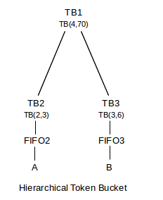
If TB1’s rate is, as here, less than the sum of its child rates, then as long as its children always have packets ready to send, the children will receive bandwidth in proportion to their token bucket rates. In the example above, TB1’s rate is 4 packets/ms and yet the sum of the rates of its children is 5 packets/ms. Each child will therefore receive 4/5 its promised rate: TB2 will send at a rate of 2×(4/5) packets/ms while TB3 will send at rate of 3×(4/5) packets/ms.

To see this, assume FIFO2 and FIFO3 remain nonempty for a period long enough for their buckets to empty. TB2 and TB3 will then each release packets to TB1 at their respective rates of 2 packets/ms and 3 packets/ms. In the following sequence of release times to TB1, we assume TB3 starts at T=0 and TB2 at T=0.01, to avoid ties. Packets from A released by TB2 are shown in italic:

0, 0.01, .33, 0.51, .67, 1.0, 1.01, 1.33, 1.51, 1.67, 2.0, 2.01

They will be dequeued by TB1 at 4 packets/ms, once TB1’s bucket is empty. In the long run, TB3 has released three packets into this sequence for every two of TB2’s, so sender B will receive 3/5 of the dequeuings, and thus 3/5 of the 4 packet/ms root bandwidth.

We can also have each token-bucket node physically forward released packets to FIFO queues attached to each parent node; we called this an internal-storage hierarchy in 17.7 Hierarchical Queuing. In this particular case, the leaf-storage and internal-storage mechanisms function identically, provided the internal links are infinitely fast and the internal queues infinitely large. See exercise 18.

There is no point in having a node with a bucket larger than the sum of its child buckets and also a rate larger than the sum of its child rates. In the example above, in which the sum of the child rates exceeds the parent rates, A would be able to send at a sustained rate of 2 packets/ms provided B sends at only 2 packets/ms as well; reducing the child rates to 2×(4/5) and 3×(4/5) packets/ms respectively is not equivalent. If a node’s rate is larger than the sum of the child rates, then it will be able to handle the child traffic without delay once the child buckets have emptied. Before that, though, the parent bucket may be the limiting factor.

17.13 Fair Queuing / Token Bucket combinations¶

At first glance, combining fair queuing with token bucket might seem improbable: the goal of fair queuing is to be work-conserving, allowing the bandwidth assigned to an idle input class to be divided among the active input classes, and the goal of token bucket is generally to limit a class to its token-bucket-defined maximum transmission rate. The usual approach to a hierarchy-based synthesis is to allow the administrator to decide, at each node of the hierarchy, whether or not the node can “borrow” (without repayment) bandwidth from inactive siblings. If it can, the set of siblings with mutual borrowing privileges resembles a fair-queuing scheduler; if not, the node is more like a token-bucket scheduler.

17.13.1 CBQ¶

CBQ was introduced in [CJ91] and analyzed in [FJ95]. It did not actually use the token-bucket mechanism, but instead implemented shaping by keeping track of the average idle time (more precisely, non-transmitting time) for a given input class. Input classes that tried to send too much were restricted, unless the node was permitted to “borrow” bandwidth from a sibling. When an input class sent less than it was allowed, its average utilization would fall; if a burst arrived then it would take some time for the average to “catch up” and thus the node could briefly send faster than its assigned rate. However, the size of the “bucket” could be controlled only indirectly.

17.13.2 Linux htb¶

The linux htb queuing discipline allows the same general functionality of CBQ, but replaces the average-idle calculations with token-bucket filters. This permits more direct control of burst sizes, and also avoided some technical timing issues that CBQ users had to watch out for. For efficiency, htb uses the quantum algorithm for fair queuing; as noted in 17.5.5 The Quantum Algorithm, this means less precise control over packet delay.

It is common to arrange for htb to apply token-bucket shaping only at the leaf nodes, and to configure the interior nodes do fair queuing only.

Each node in the tree has the following attributes:

its guaranteed rate, r, corresponding to the token-bucket rate
its burst allowance B, corresponding to the bucket size
its ceiling rate r_ceil; nodes never send faster than this

In many cases r_ceil may simply be the output rate of the root node.

The most important attribute of each node is its guaranteed rate. If inner nodes are not doing token-bucket shaping then the rate at each node should be at least as large as the sum of the child rates; in the following diagram, all rates are in Kbps. Burst allowances are not shown. We will assume the root guaranteed rate, 600 Kbps, is also its ceiling rate.

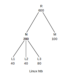
Packets are marked green, yellow or red depending on their situation. Red packets are those that must wait; eventually they will turn yellow and then green.

Packets are considered green if they are now compliant (perhaps after waiting earlier) for one of the leaf token-bucket nodes; green packets are sent as soon as possible. If the parent-node rate is at least as large as the sum of the child-node rates, the parent node will not be a bottleneck.

After L1, L2 and L3 have each emptied their buckets, they will not exhaust N’s rate. Similarly, after N and M have emptied their buckets they will use only half of R’s rate. Packets are allowed to “borrow” – without payback – from their parent’s rates; such packets are marked yellow, and may also be sent immediately if no green packets are waiting. Borrowing is always in proportion to a node’s guaranteed rate, in the manner of fair queuing. That is, the guaranteed rates of the child nodes are treated as unnormalized fair-queuing weights; normalized weight fractions are obtained by dividing by their total. N above would have normalized weight fraction 200/(200+100) = 2/3.

If L1, L2 and L3 engage in borrowing from N, and each has traffic to send, then each gets a total bandwidth of 50, 50 and 100 Kbps, respectively. If L3 is idle, then L1 and L2 each would get 100 Kbps. If N and M borrow in turn from R, they each can send at 400 and 200 Kbps respectively, in which case L1, L2 and L3 (again assuming all are active) get 100, 100 and 200 Kbps. If M elects not do do any borrowing, because it has nothing to send, then N will get 600 Kbps and L1, L2 and L3 will get 150, 150 and 300.

If fair-queuing behavior is not desired, we can set r_ceil = r so that a node can never send faster than its guaranteed rate. This allows htb to model the token-bucket-only hierarchy of 17.12 Hierarchical Token Bucket.

17.13.3 Parekh-Gallager Theorem¶

As a final example relating token-bucket specifications and fair queuing, we present the Parekh-Gallager Theorem, which provides a precise queuing-delay bound on traffic that enters a network meeting a token-bucket specification TB(r,B) and which has a guaranteed weighted-fair-queuing fraction through each router along the path.

Specifically, let us assume that the traffic travels from sender A to destination B through N routers R₁ ... R_N. The output rate of the ith router R_i is r_i, of which our flow is guaranteed rate f_i≤r_i. Let f = min {f_i|i<N}. Suppose the maximum packet size for packets in our flow is S, and the maximum packet size including competing traffic is S_max. Then the total delay encountered by the flow’s packets is bounded by the sum of the following:

propagation delay (total single-bit delay along all N+1 links)
B/f
The sum from 1 to N of S/f_i
The sum from 1 to N of S_max/r_i

The second term B/f represents the queuing delay introduced by a single burst of size B; we showed in 17.11.2 Token Bucket Through Multiple Routers that this delay bound applied regardless of the number of routers.

The third term represents the total store-and-forward delay at each router for packets belonging to our flow under GPS; the delay at R_i is S/f_i.

The final term represents the degree to which fair-queuing may delay a packet beyond the theoretical GPS time expressed in the third term. If the routers were to use GPS, then the first three terms above would bound the packet delay; we established in 17.5.4.7 Finishing-Order Bound that router R_i may introduce an additional delay above and beyond the GPS delay of at most S_max/r_i.

17.14 Epilog¶

If we want to use 100% the outbound bandwidth, but divide it among several senders according to a predetermined ratio, fair queuing is the tool to use. If we want to impose an absolute rather than a relative cap on traffic, token bucket is appropriate.

Fair queuing has applications to the routing of ordinary packets; for example, if routers implement fair queuing on a per-connection basis, then TCP senders will have no incentive to maximize queue utilization and TCP Reno will lose its competitive advantage.

It is for real-time traffic, however, that queuing disciplines such as fair queuing, token bucket and even priority queuing come into their own as fundamental building blocks. These tools allow us to guarantee a bandwidth fraction to VoIP traffic, or to allow such traffic to be sent with minimal delay. In the next chapter 18 Quality of Service we will encounter fair queuing and token-bucket specifications repeatedly.

17.15 Exercises¶

1. Suppose a router uses fair queuing with three input classes, and uses the quantum algorithm of 17.5.2 Different Packet Sizes. The first class sends packets of size 900 bytes, the second sends packets of 400 bytes, and the third sends packets of 200 bytes. List what would be sent by each flow in each of the first five rounds.

2. Suppose we attempt to simulate BBRR as follows with the following strategy we will call SBBRR. Each subqueue has a bit-position marker that advances by one bit for each bit we have available to send from that queue. If three queues are active, then in the time it takes us to send three bits, each marker would advance by one bit. When all the bits of a packet have been ticked through, the packet is sent.

(a). Explain why this is not the same as BBRR fair queuing (even with equal-sized packets).

(b). Is it the same as BBRR if all input queues are active?

3. Suppose we modify the SBBRR strategy of the previous exercise so that, if the output link is ever idle, and no packet has yet had all its bits ticked through by the bit-position marker, then we immediately send the packet with the fewest bits remaining to be ticked through by the bit-position marker.

Suppose packets P1 of size 1000 and P2 of size 100 arrive on subqueue 1. Just after P1 begins transmission, packet Q1 of size 400 arrives on subqueue 2. Fair queuing should send the packets in the order P1, Q1, P2; show that the mechanism described here does not do that.

4. Suppose we attempt to implement fair queuing by calculating the finishing time F_j for P_j, the jth packet in subqueue i, as follows.

Start_j+1 = max(F_j, now) (“now” by wallclock time)

F_j = Start_j + N×L_j

where N is the total number of subqueues, active or not.

(a). Suppose a router has three subqueues; ie N=3. The outbound bandwidth is 1 size unit / 1 time unit. At T=0, packets P1, P2, P3, P4 and P5 arrive for subqueue 1, each of size 1 unit. At T=2 (by which point P1 and P2 will have finished transmission), packets Q1 and Q2 arrive on subqueue 2, also of size 1. What finishing times will all the packets be assigned? In what order will they be transmitted?

(b). Is this strategy approximately equivalent to fair queuing if we are given that all subqueues of the router are always active?

5. Suppose we modify the strategy of the previous exercise by letting N be the number of active subqueues at the time of arrival of packet P_j. What happens if we have three input subqueues, and at T=0 five packets arrive for subqueue 1, and at T=1 five packets arrive for subqueue 2. Assume all ten packets are of size 1, and the output bandwidth is again 1 size unit per time unit.

6. The following packets all arrive at time T=0 at a router with an output rate of one size unit per time unit.

Subqueue 1: P1 of size 100, P2 of size 500, P3 of size 400

Subqueue 2: Q1 of size 300, Q2 of size 200, Q3 of size 600

Subqueue 3: R1 of size 400, R2 of size

(a). Find the BBRR virtual finishing time of each packet

(b). Give the actual wallclock finishing time of each packet, if the packets were sent via BBRR

7. Calculate GPS finishing times for the following packets, all present at T=0. There are two subqueues, and their bandwidth fractions are 𝛼 and 𝛽 where 𝛼 = (√5-1)/2 ≃ 0.618 and 𝛽 = 𝛼² = 1-𝛼. The packet sizes for the two subqueues are as follows (they follow the Fibonacci sequence, except 2 appears twice):

𝛼: 2, 3, 8, 21, 55, 144, 377, 987

𝛽: 1, 2, 5, 13, 34, 89, 233, 610

Hint: you will have to evaluate 𝛼 to more decimal places than is shown here.

8. Suppose a WFQ router has two subqueues, each with a bandwidth fraction of 𝛼=50%. The router transmits 1 byte per ms. Initially, the subqueues are empty and T=0 and the GPS virtual clock is 0. At that moment a packet P1 of size 1000 bytes arrives at the first subqueue. At T=500, a similarly sized packet P2 arrives at the second subqueue. Give, for each of P1 and P2,

(a). Its finishing time under the GPS virtual clock
(b). Its wallclock finishing time
(c). The value of the GPS virtual clock at the moment of WFQ finishing.

9. Suppose a router has three subqueues, and an outbound bandwidth of 1 packet per unit time. Twelve packets arrive at or after T=0, timed so that the router remains busy until finishing the packets at T=12.

(a). What packet arrival schedule leads to the minimum final BBRR clock value?

(b). What schedule leads to the maximum final BBRR clock value?

Hint: the rate of the BBRR clock depends only on the number of active subqueues.

10. Suppose packets from three subqueues are sent using the quantum algorithm of 17.5.5 The Quantum Algorithm. The packets are listed below in order of arrival for each subqueue, along with their lengths L; the packets are all available at time T=0. The quantum is 1000 bytes. Give the order of transmission.

Subqueue 1	Subqueue 2	Subqueue 3
P1, L=700	Q1, L=400	R1, L=500
P2, L=700	Q2, L=500	R2, L=600
P3, L=700	Q3, L=1000	R3, L=200
P4, L=700	Q4, L=200	R4, L=900

11. At Disneyland, patrons often wait in a queue that winds slowly through one large waiting room, only to feed into another queue in another room. Is this an example of hierarchical queuing, eg of one FIFO queue feeding another, without classes?

12. If two traffic streams meet token-bucket specifications of TB(r1,b1) and TB(r2,b2) respectively, show their commingled traffic must meet TB(r1+r2,b1+b2). Hint: imagine a common bucket of size b1+b2, filled at rate r1 with red tokens and at rate r2 with blue tokens.

13. For each sequence of arrival times, indicate which packets are compliant for the given token-bucket specification. If a packet is noncompliant, go on to the next arrival without decrementing the bucket.

(a). TB(1/4,5):  0, 0, 0, 2, 3, 4, 5, 7, 9, 11, 15, 18
(b). TB(1/3,6):  0, 0, 0, 1, 2, 3, 4, 5, 6, 7, 8, 9
(c). TB(1/3,6):  0, 2, 4, 6, 8, 10, 12, 14, 16, 18

14. Find the fastest sequence (see the end of 17.9.3 Multiple Token Buckets) for the following flows. Both start at T=0, and all buckets are initially full.

(a). TB(1/4, 4); packets can depart at a minimum of 1 time unit apart. Continue the sequence to at least T=10

(b). TB(1/2, 4) and TB(1/8, 8); multiple packets can depart at the same instant. Continue to at least T=25.

15. Give the fastest sequence of packets compliant for all three of the following token-bucket specifications. Continue the sequence at least until T=60.

TB(1/2, 1)
TB(1/6, 4)
TB(1/12, 8)

Hint: the first specification means arrival times must always be separated by at least 2. The middle specification should kick in by T=12.

16. Show that if a GPS traffic flow satisfies a token-bucket specification TB(r,B), then in any interval of time t₁≤t≤t₂ the amount of traffic is at most B + r×(t₂−t₁). Hint: during the interval t₁≤t≤t₂ the amount of fluid added to the bucket is exactly r×(t₂−t₁).

17. Show that a generic hierarchy of FIFO queuing disciplines, described in 17.7.1 Generic Hierarchical Queuing, collapses to a single FIFO queue.

18. Show that the token-bucket leaf-storage hierarchy of 17.12 Hierarchical Token Bucket produces the same result as an “internal-storage” hierarchy in which each intermediate token-bucket node contained a real, infinite-capacity FIFO queue, and each node instantaneously transmitted each packet to the parent’s FIFO queue as soon as it was released. Show that packets are transmitted by each hierarchy at the same times. Hint: show that each node in the leaf-storage hierarchy “releases” a packet at the same time the corresponding internal-storage hierarchy forwards the packet upwards.

19. The following linux htb hierarchies are labeled with their guaranteed rates. Is there any difference in terms of the bandwidth allocations that would be received by senders A and B?

   (a)                                 (b)
    R                                   R
   100                                 100
  /   \                               /   \
 /     \                             /     \
L1     L2                           L1     L2
60     40                           30     20
|       |                           |       |
A       B                           A       B

20. Suppose we know that the real-time traffic through a given router R uses at most 1 Mbps of the total 10 Mbps bandwidth. Consider the following two ways of giving the real-time traffic special treatment:

i. Using priority queuing, and giving the real-time traffic higher priority.

ii. Using weighted fair queuing, and giving the real-time traffic a 10% share

(a). Show that, if the real-time traffic meets a token-bucket specification with rate 1 Mbps and negligible bucket size, then the two mechanisms are equivalent, in the sense that if the real-time and non-real-time traffic flows are sending at fractions 𝛼 and 𝛽, respectively, of the 10 Mbps outbound rate, with 𝛼+𝛽=1 (and with 𝛼≤10%), then the two methods above will actually send at the same rates.

(b). What differences can be expected if the bucket size is not negligible? Which approach will favor the real-time fraction?

21. In the previous exercise, now suppose we have two separate real-time flows, each guaranteed by a token-bucket specification not to exceed 1 Mbps. Is there a material difference between any pair of the following?

i. Sending the two real-time flows at priority 1, and the remaining traffic at priority 2.

ii. Sending the first real-time flow at priority 1, the second at priority 2, and the remaining traffic at priority 3.

iii. Giving each real-time flow a WFQ share of 10%, and the rest a WFQ share of 80%

Navigation

Table Of Contents

Previous topic

Next topic

Quick search